The Dynamic Segmentation pattern alters the calculation of one or more measures by grouping data according to specific conditions, typically range boundaries for a numeric value, defined in a parameter table (see the Parameter Table pattern). Dynamic segmentation uses the columns of the parameter table to define the clusters. The grouping is dynamically evaluated at query time, considering some or all of the filters applied to other columns in the data model. Thus, the parameter table and its segment name column are visible to the client tools.

If you need to store the result of a segmentation in a calculated column, refer to the Static Segmentation pattern.

Basic Pattern Example

Suppose you want to slice data by price, grouping price values in ranges that you can customize by changing a configuration table. Every price can belong to one or more groups. With dynamic segmentation, if the user selects more than one group, you still count each price only once. Thus, the resulting measure is non-additive.

To do that, you first create a Ranges table that does not have any relationship with other tables in the data model. The example in Figure 1 shows an overlap between the MEDIUM and TOP price ranges, defined by prices within 10 and 100.

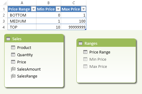
The measures you want to segment have to evaluate only the rows with a price within the selected segments. Thus, assuming that SalesAmount is the original measure, you define the corresponding SalesRange measure that handles segmentation as follows:

SalesRange :=
CALCULATE (
    [SalesAmount],
    FILTER (
        VALUES ( Sales[Price] ),
        COUNTROWS (
            FILTER (
                Ranges,
                Sales[Price] >= Ranges[Min Price]
                && Sales[Price] < Ranges[Max Price]
            )
        ) > 0
    )
)

The SalesRange measure defined in this way handles multiple selection within the Ranges table. However, this calculation may have some performance penalty. You can find a faster calculation that handles only single selections later, in the Complete Pattern section.

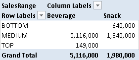
You can use such a measure in a PivotTable. For example, Figure 2 shows a PivotTable where the TOP segment contains sales in a price (14.90 per unit) that belongs to both MEDIUM and TOP ranges. In the calculation for Grand Total, such sales are considered only once, so the Grand Total corresponds to MEDIUM range.

The Dynamic Segmentation pattern can be used in a more complex way by filtering data in an entity table (such as Products or Customers) instead of directly filtering data in the fact table.

Use Cases

You can use the Dynamic Segmentation pattern any time you need to evaluate a measure and group its results dynamically into discrete clusters, using a configuration table to define the number and the boundaries of the groups. With dynamic segmentation, each entity can belong to more than one cluster (this is not possible in static segmentation). This technique is also known as dynamic banding.

Classify Items by Measure

You can apply the Dynamic Segmentation pattern to a table that represents an entity, such as Products or Customers. In a star schema, usually the entity is stored in a dimension table. But if the entity you want to group (for example, an invoice identifier) is stored in a fact table containing transactions, you can apply the measure to that table. You can use any measure to define the segment ownership of an entity. A few practical examples are:

Group Products by Sales Amount, by Margin, by Price
Group Customers by Sales Amount, by Margin, by Age
Group Countries by Sales Amount, by Margin, by Population
Group Sales by Invoice Amount

Complete Pattern

Add a Segments table to the data model, as shown in Figure 3. That table has no relationships with other tables, and usually has at least three columns: the range description and the minimum and maximum values for the range. You might use another column to specify a particular display order by using the Sort By Column property (in the example, the Segment Name is sorted by Segment Position). You should hide the Min Value and Max Value columns by using the Hide From Client Tools command on these columns (available in either Grid or Diagram view).

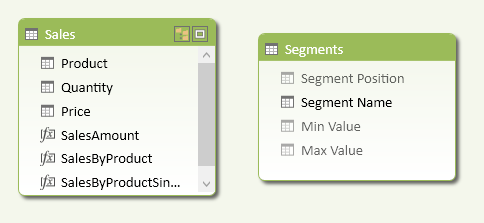
You create a measure (SalesByProduct in the Sales table in Figure 3) that evaluates the corresponding segment for each row of the table containing the entity to segment (in this case, you group products by SalesAmount).

SalesByProduct :=
IF (
    ISFILTERED ( Segments[Segment Name] ),
    CALCULATE (
        [SalesAmount],
        FILTER (
            VALUES ( Sales[Product] ),
            COUNTROWS (
                FILTER (
                    Segments,
                    [SalesAmount] >= Segments[Min Value]
                    && [SalesAmount] < Segments[Max Value]
                )
            ) > 0
        )
    ),
    [SalesAmount]
)

Such a measure evaluates the expression in a CALCULATE function that filters the entities that have to be grouped in the selected segments. The outermost FILTER iterates the list of products, whereas the innermost FILTER iterates the selected segments, checking whether the product falls within the range of at least one segment. In this way, every product can belong to zero, one, or more segments. If a product has a SalesAmount that is not included in any segment, you do not get an error. The outermost IF function checks whether there is a selection active on Segment Name, so that no segmentation will occur if there is no selection over Segments. Thus, the Grand Total in a PivotTable will contain all the data even if there are products that do not belong to any segment.

Handling the multiple selection of segments might slow the calculation, so you might use a faster algorithm that works with only one segment selected and returns BLANK when two or more segments are selected.

SalesByProductSingle:=
IF (
    ISFILTERED ( Segments[Segment Name] ),
    IF (
        HASONEVALUE ( Segments[Segment Name] ),
        CALCULATE (
            [SalesAmount],
            FILTER (
                VALUES ( Sales[Product] ),
                [SalesAmount] >= VALUES ( Segments[Min Value] )
                    && [SalesAmount] < VALUES ( Segments[Max Value] )
            )
        ),
        BLANK ()
    ),
    [SalesAmount]
)

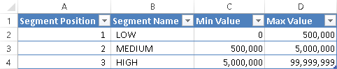
Figure 4 shows an example of a Segments table containing segments with non-overlapping ranges for SalesAmount, as specified by the Min Value and Max Value columns.

You see in Figure 5 that the SalesByProduct and SalesByProductSingle measures (as defined above) produce the same result if there is a single selection of segment.

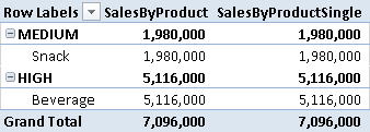
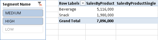
Figure 6 shows that with multiple selection of segments, the SalesByProductSingle measure always returns a blank value, whereas the SalesByProduct measure produces a correct result—one that considers the union of selected segments.

More Pattern Examples

In this section, you will see a few examples of the Dynamic Segmentation pattern.

Dynamically Group Customers by Sales Amount

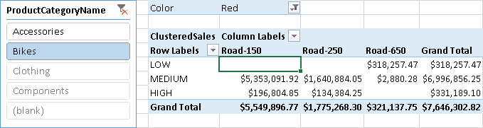
You can dynamically create groups of customers by using a measure such as SalesAmount. In each query, every customer belongs to just one group; the calculation will apply slicers and filters to measure evaluation but ignore entities put in rows and columns of a PivotTable. For example, Figure 7 shows three clusters (LOW, MEDIUM, and HIGH) of customers grouped by the amount of sales of red bikes. The clusters do not consider the product model (in columns), but filter the SalesAmount by using the ProductCategoryName selection in the slicer and the Color selection in the PivotTable filter.

The Clusters table in Figure 8 has no overlaps between ranges, but you can define a Clusters table with overlapping ranges.

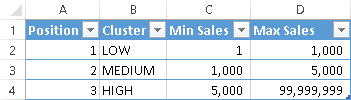
The Clusters table has no relationship with other tables in the data model. Figure 9 shows the tables imported from Adventure Works, including Products, Customers, and Sales.

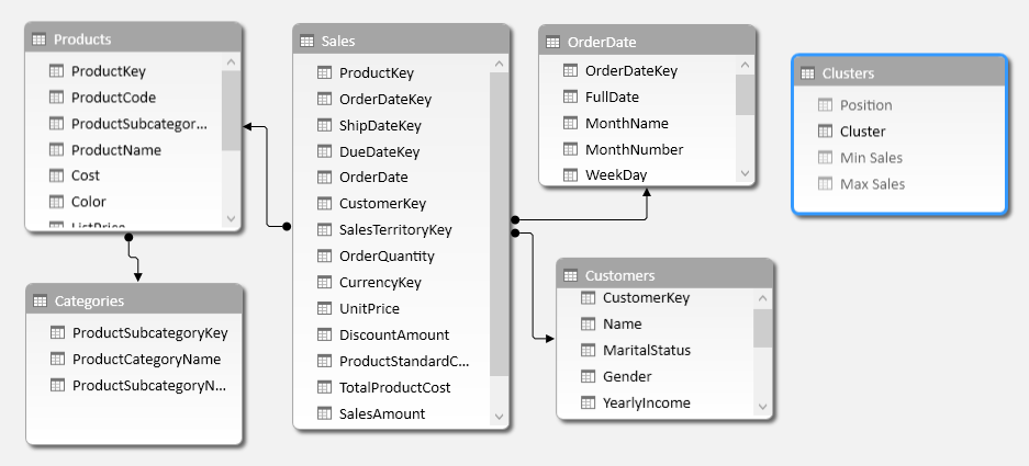
In this case, the entity used to define the clusters (Customers) is in a table related to the Sales table, which contains the columns used to compute the measure (SalesAmount). Thus, the ClusteredSales measure that computes the value using the selected clusters has to use a more complex FILTER function inside the CALCULATE function: for each customer, it has to evaluate the sum of SalesAmount applying existing filters and slicers, but removing all the filters defined in rows and columns. The ALLSELECTED function has exactly this purpose. The ClusteredSales measure is shown below.

ClusteredSales :=
CALCULATE (
    SUM ( Sales[SalesAmount] ),
    FILTER (
        ADDCOLUMNS (
            Customers,
            "CustomerSales",
            CALCULATE (
                SUM ( Sales[SalesAmount] ),
                CALCULATETABLE ( Customers ),
                ALLSELECTED ()
            )
        ),
        COUNTROWS (
            FILTER (
                'Clusters',
                [CustomerSales] >= 'Clusters'[Min Sales]
                && [CustomerSales] < 'Clusters'[Max Sales] 
            ) 
        ) > 0
    )
)

There is another important note in the previous formula. You have to evaluate the sum of the SalesAmount measure for each customer in the iteration defined by the ADDCOLUMNS function. The CALCULATE statement (passed as an argument to ADDCOLUMNS) transforms the row context (on Customers) into a filter context. However, the presence of ALLSELECTED in the CALCULATE function would remove the filter context (from Customers) obtained by the row context. To restore it, a CALCULATETABLE statement (on Customers) is included in another argument, so that the “current” customer is added to the filter context again. Without this CALCULATETABLE function, the result in Figure 7 would have put all the customers in the same cluster (HIGH), considering the total of all the customers for each customer during the iteration made by the ADDCOLUMNS function.

You can see the list of customers belonging to each cluster by putting the customer names in rows under the cluster Name. If you have no overlapping segments, every customer will be included in only one cluster, as you see in Figure 10.

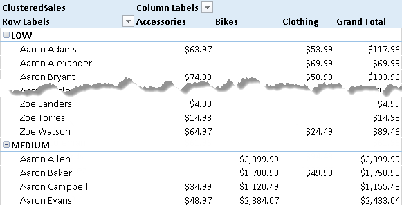
Please note that without the ALLSELECTED function called in the CALCULATE statement for the CustomerSales calculated field, the cluster evaluation would happen cell by cell, and the same customer might belong to several clusters. For example, without ALLSELECTED, the clusters in Figure 10 would be computed considering the sales of each product category, which appear on columns, instead of the sales of all the products for each customer, as shown.