The dynamic version of the ABC Classification pattern is an extension of the Dynamic Segmentation pattern. It groups items (such as Products or Customers) into segments based on their cumulated sales and how much they contributed to the total sales across all items. Dynamic segmentation is calculated on the fly with respect to all the filters, unlike the static ABC Classification pattern, where segments are calculated during processing and are therefore independent of any filters later applied to the pivot table. Dynamic segmentation allows you to analyze how a specific item varies across regions or has moved between classes over time. In the pattern, you use a parameter table to define the boundaries of the different segments (see the Parameter Table pattern).

Before advancing with this pattern, please make sure that you are already familiar with the following patterns:

Basic Pattern Example

Suppose that, in addition to analyzing the overall importance of a certain product in terms of ABC Classification, you also want to analyze the development of this product over time. In this case, you need a dynamic approach that does the segmentation separately for each time period. The general approach is the same as for the static ABC Classification, but now we calculate the segmentation on the fly in the context of all current filters. The final calculation is very flexible and works with any filter.

The data model shown in Figure 1 contains the following tables:

Sales: product sales on granularity of product, date, and sales territory.
Products: items subject to ABC classification.
Date: days, months, and years used for order date.
SalesTerritory: regions where the products are sold.
Classifications: classes and their boundaries.

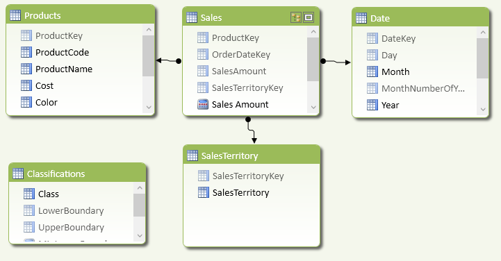
Note that the Classifications table does not have relationships with any other table. You will use a virtual relationship in the DAX calculation for the segmentation.

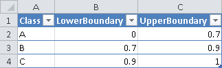
The Classifications table contains the values you can see in Figure 2.

The dynamic ABC Classification requires the definition of these four measures:

Sales Amount: the sales on which the calculation will be based.
MinLowerBoundary: the lower boundary of the currently selected segment.
MaxUpperBoundary: the upper boundary of the currently selected segment.
Sales Amount ABC: the final measure that groups the single items into segments based on their cumulated sales.

Sales Amount := 
SUM ( 'Sales'[SalesAmount] )

MinLowerBoundary := 
MIN ( 'Classifications'[LowerBoundary] )

MaxUpperBoundary :=  
MAX ( 'Classifications'[UpperBoundary] )

Sales Amount ABC :=
CALCULATE (
    [Sales Amount],
    VALUES ( 'Products'[ProductCode] ),
    FILTER (
        CALCULATETABLE (
            ADDCOLUMNS (
                ADDCOLUMNS (
                    VALUES ( 'Products'[ProductCode] ),
                    "OuterValue", [Sales Amount]
                ),
                "CumulatedSalesPercentage", DIVIDE (
                    SUMX (
                        FILTER (
                            ADDCOLUMNS (
                                VALUES ( 'Products'[ProductCode] ),
                                "InnerValue", [Sales Amount]
                            ),
                            [InnerValue] >= [OuterValue]
                        ),
                        [InnerValue]
                    ),
                    CALCULATE (
                        [Sales Amount],
                        VALUES ( 'Products'[ProductCode] )
                    )
                )
            ),
            ALL ( 'Products' )
        ),
        [CumulatedSalesPercentage] > [MinLowerBoundary]
            && [CumulatedSalesPercentage] <= [MaxUpperBoundary]
    )
)

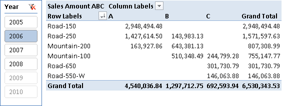
You can now use the Class column from the Classifications table together with the Sales Amount ABC measure to display the segments and their values. By further adding a slicer for the year, you can filter by Year(s) and recompute the classification based on the existing slicer selection. Thus, both the classification and the Sales Amount ABC measure are calculated with respect to the selected filter(s), as shown in Figure 3.

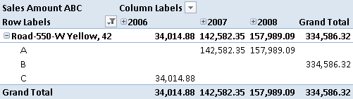
In Figure 4 you can see how a single product moves between segments over time.

The dynamic ABC Classification pattern is used to group items (such as Products or Customers) after they have been filtered by a given criteria. Usually, you use this classification in combination with time or region to find important items for a given selection.

Use Cases

In addition to all use cases that the static ABC Classification pattern covers (such as inventory management, customer segmentation, and marketing segmentation), the dynamic calculation further extends the pattern’s analytical capabilities by allowing slicing and dicing by all the other dimensions and hierarchies.

Track Product or Customer Performance Over Time

You can use the dynamic version of ABC Classification to track the performance of a product or set of products over time. This allows early identification of their declining or increasing importance for the business. This information can then be used to start a marketing campaign or to remove a product from sale.

Compare Product Performance Across Regions

You can identify regional differences between products and sets of products in terms of sales by using dynamic ABC Classification. This allows you to prioritize certain products and/or regions for sales and marketing, or simply helps you analyze data by region to understand your business better.

Complete Pattern

You can apply the dynamic ABC Classification pattern to any existing data model. It does not require any special arrangement of the data model; you will only need to add a table that defines the ABC segments and their boundaries.

First, you have to identify the measure to use for the segmentation. Such a measure must aggregate by using the SUM function in order for the dynamic ABC Classification pattern to work properly. A typical example would be the sum of sales.

<segmentation_measure> :=
SUM ( '<fact_table>'[<value_column>] )

The next step is to identify the table that contains the items to classify. This is the . The identifies the column of the item table corresponding to its business key (e.g., customer number or product code).

You add a table () that defines classes and boundaries. You have seen an example of this table in Figure 2. This table contains three columns:

<class>: name of the segment (usually A, B, and C).
<lower_boundary>: the lower boundary of the segment in percent (0.7 means 70%).
<upper_boundary>: the upper boundary of the segment in percent (0.9 means 90%).

You create the following measures to calculate the values of the boundaries for the currently selected segment:

[MinLowerBoundary] :=
MIN ( <lower_boundary> )

[MaxUpperBoundary] := 
MAX ( <upper_boundary> )

Once all these prerequisites are in place, you can create the final calculation:

<measure ABC> :=
CALCULATE (
    <segmentation measure>,
    VALUES ( <business_key_column> ),
    FILTER (
        CALCULATETABLE (
            ADDCOLUMNS (
                ADDCOLUMNS (
                    VALUES ( <business_key_column> )
                    "OuterValue", <segmentation_measure>
                ),
                "CumulatedValuePercentage", DIVIDE (
                    SUMX (
                        FILTER (
                            ADDCOLUMNS (
                                VALUES ( <business_key_column> ),
                                "InnerValue", <segmentation_measure>
                            ),
                            [InnerValue] >= [OuterValue]
                        ),
                        [InnerValue]
                    ),
                    CALCULATE ( 
                        <segmentation_measure>, 
                        VALUES ( <business_key_column> )
                    )
                )
            ),
            ALL ( <item_table> )
        ),
        [CumulatedValuePercentage] > [MinLowerBoundary]
            && [CumulatedValuePercentage] <= [MaxUpperBoundary]
    )
)

The final formula is rather complex. In order to make it easier to understand, let us break it down into separate logical steps.

First, you have to define the set of items that are relevant for the segmentation. This is done using CALCULATETABLE with a specific filter—e.g., ALL() to consider all items. Later in this pattern, you will learn how you can modify this filter to achieve different results according to your requirements.
Once you have the set of items, you have to calculate the cumulated sales for each item. This is a two-step process:
- Get the current value for each item. In our formula, this is the OuterValue column, which is calculated for every item in the current filter using ADDCOLUMNS and VALUES.
- Calculate the cumulated value for each item by iterating over the full item-table again, and sum up all the values that are greater than or equal to the OuterValue calculated in the previous step. This is the SUMX over the FILTER part.
You divide the cumulated sales by the total value over all relevant items to get the cumulated percentage of total (CumulatedValuePercentage) for each item. We are using DIVIDE for this purpose.
The resulting table contains each item and its CumulatedValuePercentage. Then, you filter this table by the boundaries of the current segment’s boundary values, returning a table that only contains items falling into the current segment.
The outermost CALCULATE function uses this result as a table filter and limits the calculation to only items in the current segment.
As the table filter would overwrite any existing filters on our business key column (e.g., if the business key column was used on rows), we need to add VALUES() in order to retain the current filter context on the business key column.

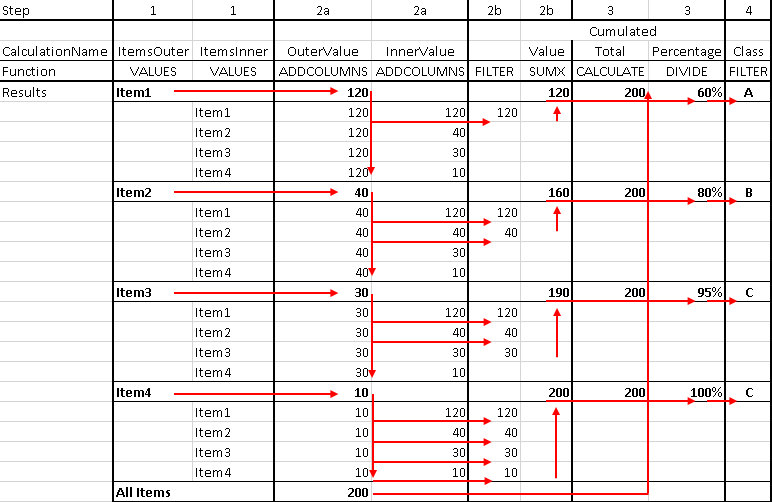
Figure 5 illustrates the different steps of the evaluation process that performs the full operation of segmenting products and then calculating cumulated sales. The calculation order is from left to right.

Pattern Variations

You can change the ABC Classification pattern to fit specific needs. There are two common variations in a real-world scenario.

Dynamic Classification on Page-Filter Level

The basic ABC Classification (dynamic) pattern calculates the segments for each slice of the result set. For example, if you have years in columns, the segmentation is done for each year, as shown above in Figure 4. This way you can track performance of a single item over years. However, for some scenarios you might want to do the segmentation only in the context of the page filters, using the same segmentation for all the columns. For example, in Figure 6 you split sales of each segment over different regions.

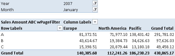
As you can see, in North America, products in segment C are performing better than those in segment B. This is because the products are associated to the segments based on the value of the Grand Total column, where you can see the 70/20/10 split of ABC classification. A product with good total sales across all the continents (Grand Total) might have lower sales in a single region (e.g., North America). This type of segmentation can lead to valuable insights for marketing and sales departments.

In order to obtain this result, you add ALLSELECTED to the filter arguments of the CALCULATETABLE function:

Sales Amount ABC wPageFilter :=
CALCULATE (
    <classification_measure>,
    VALUES ( <business_key_column> ),
    FILTER (
        CALCULATETABLE (
            ADDCOLUMNS (
                ADDCOLUMNS (
                    VALUES ( <business_key_column> )
                    "OuterValue", <segmentation_measure>
                ),
                "CumulatedSalesPercentage", DIVIDE (
                    SUMX (
                        FILTER (
                            ADDCOLUMNS (
                                VALUES ( <business_key_column> ),
                                "InnerValue", <segmentation_measure>
                            ),
                            [InnerValue] >= [OuterValue]
                        ),
                        [InnerValue]
                    ),
                    CALCULATE ( 
                        <segmentation_measure>, 
                        VALUES ( <business_key_column> )
                    )
                )
            ),
            ALL ( <item_table> ),
            ALLSELECTED ( )
        ),
        [CumulatedSalesPercentage] > [MinLowerBoundary]
            && [CumulatedSalesPercentage] <= [MaxUpperBoundary]
    )
)

Dynamic Classification Within Groups

There might be scenarios where you first want to group your items and then do the segmentation within those groups. Suppose your products belong to different business areas, and you want to do a segmentation within those areas because the products themselves are independent of each other. For example, the pivot table in Figure 7 shows the segmentation within a particular group (the color Multi).

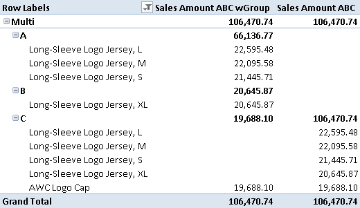
Across all groups, all the Multi-color items are in segment C (see values in the Sales Amount ABC column), because by default the segmentation applies to products of any color. However, you can do the segmentation within selected groups (e.g., products of Multi color) as shown in the Sales Amount ABC wGroup column. To do that, you change the calculation by using ALLEXCEPT instead of ALL. In this way, the segmentation happens within the currently selected group. In the following example, would be a reference to ‘Products'[Color]:

Sales Amount ABC wGroup :=
CALCULATE (
    <segmentation_measure>,
    VALUES ( <business_key_column> ),
    FILTER (
        CALCULATETABLE (
            ADDCOLUMNS (
                ADDCOLUMNS (
                    VALUES ( <business_key_column> )
                    "OuterValue", <segmentation_measure>
                ),
                "CumulatedSalesPercentage", DIVIDE (
                    SUMX (
                        FILTER (
                            ADDCOLUMNS (
                                VALUES ( <business_key_column> ),
                                "InnerValue", <segmentation_measure>
                            ),
                            [InnerValue] >= [OuterValue]
                        ),
                        [InnerValue]
                    ),
                    CALCULATE ( 
                        <segmentation_measure>, 
                        VALUES ( <business_key_column> )
                    )
                )
            ),
            ALLEXCEPT ( <item_table>, <group_column> )
        ),
        [CumulatedSalesPercentage] > [MinLowerBoundary]
            && [CumulatedSalesPercentage] <= [MaxUpperBoundary]
    )
)

Other Variations

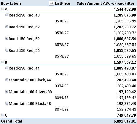
The list of variations is endless. You can use any filter by simply extending or changing the parameters of the CALCULATETABLE function. Hard-coded filters are also possible. For example, given the example in Figure 8, if you want to consider only products with a list price greater than 3,000, the would be a reference to ‘Products'[ListPrice] and the would be 3,000:

This is the corresponding pattern for this variation:

Sales Amount ABC wFixedFilter :=
CALCULATE (
    <segmentation_measure>,
    VALUES ( <business_key_column> ),
    FILTER (
        CALCULATETABLE (
            ADDCOLUMNS (
                ADDCOLUMNS (
                    VALUES ( <business_key_column> )
                    "OuterValue", <segmentation_measure>
                ),
                "CumulatedSalesPercentage", DIVIDE (
                    SUMX (
                        FILTER (
                            ADDCOLUMNS (
                                VALUES ( <business_key_column> ),
                                "InnerValue", <segmentation_measure>
                            ),
                            [InnerValue] >= [OuterValue]
                        ),
                        [InnerValue]
                    ),
                    CALCULATE ( 
                        <segmentation_measure>, 
                        VALUES ( <business_key_column> )
                    )
                )
            ),
            ALL ( <item_table> ),
            <filter_column> >= <filter_value>
        ),
        [CumulatedSalesPercentage] > [MinLowerBoundary]
            && [CumulatedSalesPercentage] <= [MaxUpperBoundary]
    )
)

ABC Classification – Dynamic