The Parameter Table pattern is useful when you want to add a slicer to a PivotTable and make it modify the result of some calculation, injecting parameters into DAX expressions. To use it, you must define a table that has no relationships with any other table. Its only scope is to offer a list of possible choices to the end user in order to alter the calculations performed by one or more existing measures.

The DAX expression in measures checks the value selected and calculates the result accordingly. In most cases, users can select only one value, and multiple selections cannot perform a meaningful calculation. For example, the Parameter Table can choose the number of customers to show in a PivotTable sorted by sales amount, similar to a dynamic “top N customers” calculation, where a slicer selects the N^th value.

Basic Pattern Example

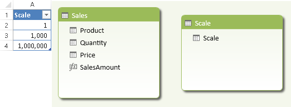
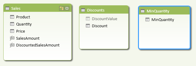
Suppose you want to provide the user with a slicer that can select the scale of measures to display, allowing the user to select a value in millions, thousands, or units. To do that, you must first create a Scale table that does not have any relationship with other tables in the data model, as shown in Figure 1.

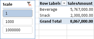
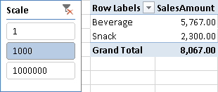
Every measure in the data model has to divide the value by the scale selected, obtaining the value from a filter context containing a single selection, as shown in Figures 2 and 3.

You define the Sales Amount measure as follows:

Sales Amount :=
IF (
    HASONEVALUE ( Scale[Scale] ),
    SUM ( Sales[SalesAmount] ) / VALUES ( Scale[Scale] ),
    SUM ( Sales[SalesAmount] )
)

This pattern is typically used when you want to inject a parameter inside a DAX measure. This example uses a scale, but you can use the same technique in many other scenarios.

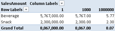
It is interesting to note that the parameter works not only with a slicer, but on rows and columns as well. For example, in Figure 4, the Scale parameter displays different values in different columns.

Use Cases

Algorithm Parameter and Simulation

You can pass one or more parameters to an algorithm by using a table for each parameter. For example, when you have a model with measures that can receive a parameter for the calculation, this pattern enables the user to change the parameters of the algorithm. This can be useful to simulate different scenarios based on different values of parameters in a simulation (e.g., discount based on volume sales level, percentage growth of revenues, drop rate in customer retention, and so on).

Algorithm Selection

You might decide to apply a different algorithm to the same measure. This means using a SWITCH statement that, according to the value selected, returns a different expression for the same measure. You will see an example later by looking at the Period Table pattern.

Ranking

You can parameterize the number of elements shown in a PivotTable according to a particular ranking. Even if you cannot define a dynamic set in DAX, you can define a measure that returns BLANK for items that you do not want to show according to the filter selected by the user. This scenario is demonstrated later in the Limit Top N Elements in a Ranking example.

Complete Pattern

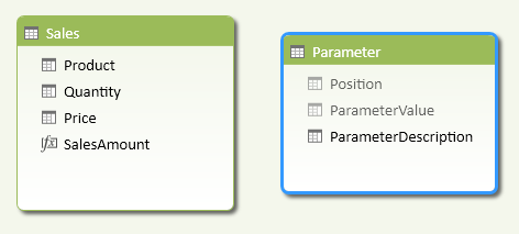
Add a Parameter table to the data model. That table has no relationships with other tables, and usually has only one column, containing the parameter values. You might use up to three columns in case you want to add a textual description to the parameter value and to specify a particular display order by using the Sort by Column property. If many parameters will be used in your data model, you can add all of them to the same table in order to reduce the number of tables in the model. You obtain such a table by performing a Cartesian product between all the possible values of each parameter (also called a cross join of parameters values). In that case, all of the columns for each parameter have to participate in the cross join.

To get the selected value, use the VALUES function in the measure that uses the parameter. Usually you check the selection of one value only. If the selection is of all the parameters, it is like there is no selection at all and, in this case, you can return a default value. If the selection has more than one but not all parameters, you might consider this case as a multiple selection, which in most cases may be an invalid selection. The following code represents the complete pattern that you see applied later in more pattern examples.

ParameterSelection :=
IF (
    HASONEVALUE ( Parameter[ParameterValue] ),
    "Selection: " & VALUES ( Parameter[ParameterValue] ),
    IF (
        NOT ( ISFILTERED ( Parameter[ParameterDescription] ) ),
        "No Selection",
        "Multiple Selection"
    )
)

It is important that you use the ISFILTERED function on the visible column, which is the one directly used by the user (ParameterDescription in the essential pattern). You have to use the VALUES function on the value column (ParameterValue in the example).

You can replace the Selection, No Selection, and Invalid Selection expressions with specific formulas that perform a meaningful calculation in each case. For example, you might return BLANK in case of multiple selection (which is an invalid one) and apply a default parameter in case of no selection, applying the selected parameter to your formula if the selection has only one value.

More Pattern Examples

In this section, you see a few examples of the Parameters Table pattern.

Using a Single Parameter Table

You use a Single Parameter Table pattern to apply a discount to an existing Sales Amount measure, by creating a table in your model with the values that the user will select. For example, you can add the following table to your data model, without creating any relationship between this table and other tables in the same model. The Discounts table in Figure 6 shows the possible discount percentages applicable to the sales amount.

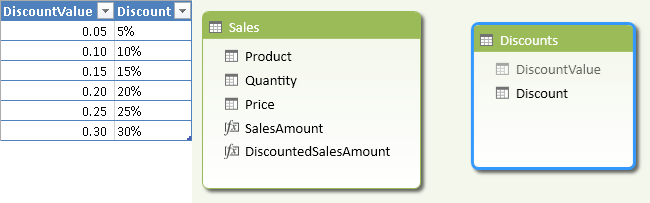
The original Sales Amount formula simply multiplies Quantity by Price for each row in the Sales table and sums the total.

SalesAmount := SUMX ( Sales, Sales[Quantity] * Sales[Price] )

The Discounted Sales Amount has to apply the selected discount to the Sales Amount measure. In order to do that, you use the VALUES function and check that the selection has only one value before evaluating the expression. If the selection includes all the discounts, you do not apply any discount, whereas if the selection includes more than one (but not all) discounts, you return BLANK.

DiscountedSalesAmount :=
IF (
    HASONEVALUE ( Discounts[DiscountValue] ),
    [SalesAmount] * ( 1 – VALUES ( Discounts[DiscountValue] ) ),
    IF (
        NOT ( ISFILTERED ( Discounts[Discount] ) ),
        [SalesAmount],
        BLANK ()
    )
)

The reason why the user can select all the values is that if there is no selection on the Discount slicer, or the user does not use the Discount attribute in the PivotTable, then all the values from Discount will appear as selected; in this scenario, it is important to provide a default value.

The HASONEVALUE function checks that the selection has only one discount. If this is not true, ISFILTERED checks whether the Discount column is part of the filter or not. If it is not in the filter, you evaluate the original SalesAmount measure; otherwise, you return BLANK because there is a selection of multiple discounts that is ambiguous.

In Figure 7, you see the PivotTable computed without selecting any discount: the two measures, SalesAmount and DiscountedSalesAmount, show the same value because the user did not apply any discount to the second measure.

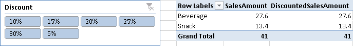
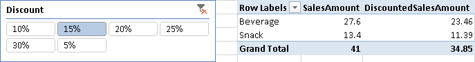
Figure 8 shows the PivotTable after selecting a 15% discount: the DiscountedSalesAmount now has a lower value than SalesAmount.

Handling More Parameter Tables

You can apply the same pattern for a single parameter table multiple times. Applied in this way, however, parameters will be independent of each other—you can neither define cascading parameters nor create constraints between combinations of parameters that are not allowed. In such a case, consider using a single column that offers only valid combinations of multiple parameter values (see an example in the section Alternative to Cascading Parameters). Every parameter requires a separate table without any relationship with other tables.

For example, you can apply the discount percentage shown in the previous section only for those sales having a minimum quantity selected through another slicer. Thus, the minimum quantity valid for applying the discount is another parameter. Figure 9 shows the resulting PivotTable with the 15% discount applied only to sales rows with a quantity greater than or equal to 3.

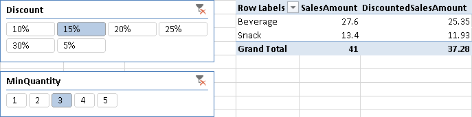
In this case, you need to create a table with one column (MinQuantity), with no relationships with other tables. The MinQuantity table contains all the numbers between 1 and 5.

In the Discounted Sales Amount measure you check the selection made on the Discounts and MinQuantity tables and, depending on that selection, you perform the right calculation. At first, it might seem necessary to use a SUMX with an IF statement in the formula, such as:

SUMX (
    Sales,
    [SalesAmount]
    * IF (
         Sales[Quantity] >= VALUES ( MinQuantity[MinQuantity] ),
         1 – VALUES ( Discounts[DiscountValue] ),
         1
      )
)

However, because the percentage will always be the same for all the discounted rows, you can also sum the result of two different CALCULATE functions:

CALCULATE (
    [SalesAmount] * ( 1 – VALUES ( Discounts[DiscountValue] ) ),
    Sales[Quantity] >= VALUES ( MinQuantity[MinQuantity] )
)
+ CALCULATE (
    [SalesAmount],
    Sales[Quantity] < VALUES ( MinQuantity[MinQuantity] )
)

The complete measure for Discounted Sales Amount is shown below. It includes the required checks for Discounts and MinQuantity selections, returning a BLANK if the user selected more than one but not all of the items in the Discounts and MinQuantity tables.

DiscountedSalesAmount :=
IF (
    HASONEVALUE ( Discounts[DiscountValue] ) && HASONEVALUE ( MinQuantity[MinQuantity] ),
    CALCULATE (
        [SalesAmount] * ( 1 – VALUES ( Discounts[DiscountValue] ) ),
        Sales[Quantity] >= VALUES ( MinQuantity[MinQuantity] )
    )
    + CALCULATE (
        [SalesAmount],
        Sales[Quantity] < VALUES ( MinQuantity[MinQuantity] )
    ),
    IF (
        NOT ( ISFILTERED ( Discounts[Discount] ) )
            && NOT ( ISFILTERED ( MinQuantity[MinQuantity] ) ),
        [SalesAmount],
        IF (
            HASONEVALUE ( Discounts[Discount] )
                && NOT ( ISFILTERED ( MinQuantity[MinQuantity] ) ) ,
            CALCULATE ( [SalesAmount] * ( 1 – VALUES ( Discounts[DiscountValue] ) ) ),
            BLANK ()
        )
    )
)

Alternative to Cascading Parameters

By using Excel slicers, you cannot show two parameters to the user in the form of cascading parameters, in which requesting the first parameter restricts the available options for the second parameter. You can partly work around this limitation by placing all cascading parameters in the same table, creating one row for each valid combination of parameters. Then, either you can display one slicer with a single description of the combination of the parameters, or you can display two or more slicers hiding the values not compatible with the current selection in other slicers.

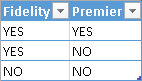
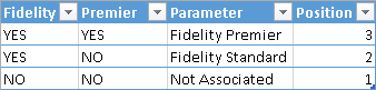
Consider two flags, one that applies a discount simulation if customers have a fidelity card and the other that simulates a further discount if customers belong to a premier level of the fidelity card. The table in Figure 11 defines the two parameters, where the combination NO/YES is not valid.

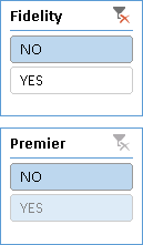
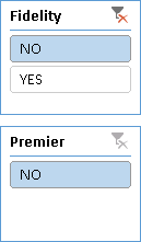
If the user selects NO in the Fidelity slicer, the Premier slicer shows the YES option even if it is not a valid combination, as shown in Figure 12.

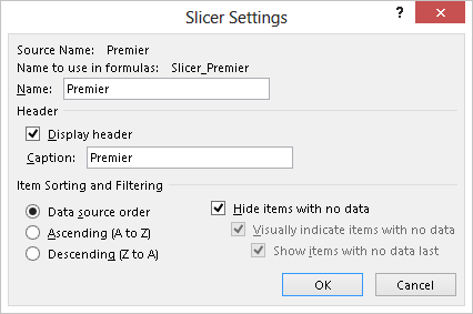
To hide the YES option in the Premier slicer when the user selects the NO value in the Fidelity slicer, use the Slicer Settings dialog box, as shown in Figure 13. In the settings for the Premier slicer, check the Hide Items With No Data checkbox.

With such a setting, the Premier slicer no longer displays the YES option when the user selects the NO value in the Fidelity slicer, as shown in Figure 14.

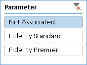
An alternative approach is to create a column that contains the description of each valid combination of parameters. By making this column visible and hiding the others, the user will be able to choose only a valid combination of parameters. As shown in Figure 15, you can use the Position column to define the sort order of the Parameter column.

The Parameter slicer shows only the valid selections in the proper sort order.

The drawback in this scenario is that a multiple selection of items in the same slicer is not meaningful. Unfortunately, it is not possible to force single selection for a slicer, so it is up to the measure expression to identify such a condition. The measures shown below return the selected value for Fidelity and Premier parameters, respectively. Before returning the value, they check the single selection of the Parameter column—if there is no selection or a multiple selection, they return a BLANK value.

FidelitySelection :=
IF (
    HASONEFILTER ( Parameters[Parameter] ),
    VALUES ( Parameters[Fidelity] ),
    BLANK ()
)
PremierSelection :=
IF (
    HASONEFILTER ( Parameters[Parameter] ),
    VALUES ( Parameters[Premier] ),
    BLANK ()
)

You can use the FidelitySelection and PremierSelection measures in other DAX expressions in order to execute algorithms according to the choice made by the user.

Period Table

As you read in other patterns, DAX provides several time intelligence functions useful for calculating information such as year-to-date, year-over-year, and so on. One drawback is that you have to define one measure for each of these calculations, and the list of measures in your model might grow too much.

A possible solution to this issue is to create a parameter table that contains one line for each calculation that you might want to apply to a measure. In this way, the end user has a shorter list of measures and possible operations on them, instead of having the Cartesian product of these two sets. This solution has its own drawbacks, however, and it may be better to create just the measures you really want to use in your data model, trying to expose only the combinations of measures and calculations that are meaningful for the expected analysis of your data.

If you decide to create a parameter table of calculations, the first step is to add a Period table in the Tabular model containing the list of possible calculations for a measure, as shown in Figure 17.

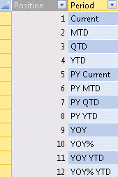
In the Period table, the Position column is hidden and the Period column has the Sort By Column set to Position. As for any parameters table, you do not have to define any relationship between this table and other tables in your data model, because you use the selected item of the Period table to change the behavior of a measure through its DAX definition.

At this point, you define a single measure that checks the selected value of the Period table and uses a DAX expression to return the corresponding calculation. Because the Period table has no relationships, when the table is used as a filter the selected value in the Period table is always the one chosen by the user. Similarly, when the Period table is used in row or column labels in a PivotTable, the selected value is the corresponding value in a row or a column. In general, you follow this generic pattern:

IF (
    HASONEVALUE ( Period[Period] ),
    SWITCH (
        VALUES ( Period[Period] ),
        "Current", <expression>,
        "MTD", <expression>,
        …

The first condition checks that there are no multiple values active in the filter context. Then, in the next step, a SWITCH statement checks each value and evaluates the correct expression corresponding to the Period value. Assuming you already defined the necessary measures for time intelligence operations, you need to replace the expression tag with the corresponding specific measure. For example, you can define a generic Sales measure, which applies one of the operations described in the Period table to the Internet Total Sales measure:

Sales :=
    IF (
        HASONEVALUE ( Period[Period] ),
        SWITCH (
            VALUES ( Period[Period] ),
            "Current", [Internet Total Sales],
            "MTD", [MTD Sales],
            "QTD", [QTD Sales],
            "YTD", [YTD Sales],
            "PY Current", [PY Sales],
            "PY MTD", [PY MTD Sales],
            "PY QTD", [PY QTD Sales],
            "PY YTD", [PY YTD Sales],
            "YOY", [YOY Sales],
            "YOY%", [YOY Sales%],
            "YOY YTD", [YOY YTD Sales],
            "YOY% YTD", [YOY YTD Sales%],
            BLANK ()
        ),
        [Internet Total Sales]
    )

Important
The RTM version of Analysis Services 2012 has an issue in SWITCH implementation, which internally generates a series of nested IF calls. Because of a performance issue, if there are too many nested IF statements (or too many values to check in a SWITCH statement), there could be a slow response and abnormal memory consumption. Service Pack 1 of SQL Server 2012 and PowerPivot 2012 fixed this issue. This is not an issue in Excel 2013.

You have to repeat such a definition for each of the measures to which you want to apply the Period calculations. You can avoid defining all the internal measures by replacing each measure’s reference with its corresponding DAX definition. This would make the Sales definition longer and hard to maintain, but it is a design choice you might follow.

Tip
Remember that you can hide a measure by using the Hide From Client Tool command. If you do not want to expose internal calculations, you should hide all the measures previously defined and make only the Sales measure visible.

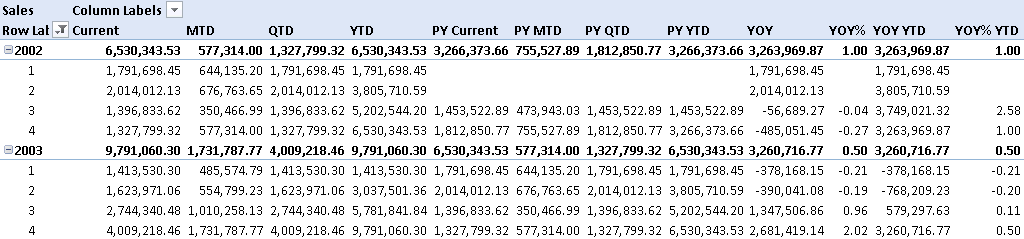
At this point, you can browse data by using the Period values crossed with the Sales measure. In Figure 18, the user displayed only the Sales measure; the Period values are in the columns, and a selection of years and quarters is in the rows.

As anticipated, this solution has several drawbacks:

After you put Period in rows or columns, you cannot easily change the order of its items. You can change the order by using some Excel features, but it is not as immediate and intuitive as changing the Position value in the Period view used to populate the Period table.
The number format of the measure cannot change for particular calculations requested through some Period values. For example, in Figure 18, you can see that the YOY% and YOY% YTD calculations do not display the Sales value as a percentage, because you can define a single number format for a measure in SSAS Tabular and you cannot dynamically change it by using an expression (as you can do in SSAS Multidimensional with MDX). A possible workaround is changing the number format directly in the client tool (Excel cells in this case), but you will lose the formatting as soon as you navigate into the PivotTable. Another workaround is returning the value as a formatted string, but the drawback in this case is that the client can no longer customize the formatting and the value is no longer a number, so it is harder to use it in further calculations in Excel.
If you use more than one measure in the PivotTable, you must create a set by using the Manage Sets command in Excel based on column items, choosing only the combination of measures and Period values that you really want to see in the PivotTable.
You have to create a specific DAX expression for each combination of Period calculations and measures that you want to support. This is not flexible and scalable as a more generic solution could be.

You have to evaluate case by case whether or not these drawbacks make the implementation of a Period table a good option.

Limit Top N Elements in a Ranking

You can easily choose the number of rows to display in a PivotTable by leveraging the TOPN function. By default, the PivotTable hides rows containing BLANK values for all the columns, so you can return BLANK for a measure that belongs to an item that is over the limit you define in the parameter. For example, if you want to display only the top 10 products by Sales Amount, you can write the Sales Amount measure in this way:

Top10SalesAmount :=
IF (
    HASONEVALUE ( Sales[Product] ),
    IF (
        RANKX (
            ALL ( Sales[Product] ),
            [SalesAmount]
        ) <= 10,
        [SalesAmount],
        BLANK ()
    )
)

You can replace the value shown in highlighted row (10) with the selection of a parameter table, as in the previous example. Of course, you always have to check for the single selection made by the user in the filter or slicer for the parameter value.

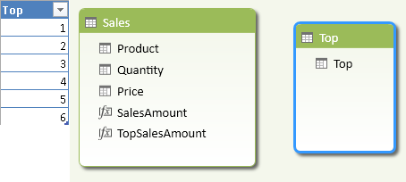
Consider the data model in Figure 19, in which the Top table contains a single column with the possible selection for the TOP N elements in the ranking.

In order to show the TOP N products, the TopSalesAmount measure compares the value returned by the RANKX function with the selected parameter and returns BLANK for the products that are outside the TOP N range.

TopSalesAmount :=
IF (
    HASONEVALUE ( 'Top'[Top] ),
    IF (
        RANKX (
            ALL ( Sales[Product] ),
            [SalesAmount]
        ) <= VALUES ( 'Top'[Top] ),
        [SalesAmount],
        BLANK ()
    )
)

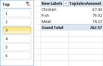
Thanks to the default PivotTable behavior, a user browsing the data model in Excel will see only the first N products after selecting a value in the Top slicer. In the example in Figure 20, there is no relationship between the sort order of the displayed products and the filter (in this case, you see the Products sorted alphabetically).

Note that this pattern assumes that a BLANK value for the measure hides a product in the report. This assumption could be false—if you select other measures in the same PivotTable or if you use other client tools to browse the data model, a product with BLANK values could be visible anyway.