Time Patterns

The DAX time patterns are used to implement time-related calculations without relying on DAX time intelligence functions. This is useful whenever you have custom calendars, such as an ISO 8601 week calendar, or when you are using an Analysis Services Tabular model in DirectQuery mode.
Basic Pattern Example
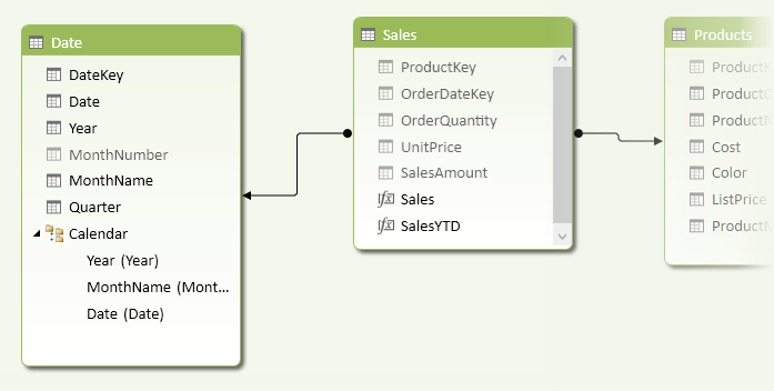
Suppose you want to provide the user with a calculation of year-to-date sales without relying on DAX time intelligence functions. You need a relationship between the Date and Sales tables, as shown in Figure 1.
The Sales measure simply calculates the sum of the SalesAmount column:
Sales := SUM ( Sales[SalesAmount] )
The year-to-date calculation must replace the filter over the Date table, using a filter argument in a CALCULATE function. You can use a FILTER that iterates all the rows in the Date table, applying a logi-cal condition that returns only the days that are less than or equal to the maximum date present in the current filter context, and that belong to the last selected year.
You define the SalesYTD measure as follows:
[SalesYTD] :=
CALCULATE (
    [Sales],
    FILTER (
        ALL ( 'Date' ),
        'Date'[Year] = MAX ( 'Date'[Year] )
            && 'Date'[Date] <= MAX ( 'Date'[Date] )
    )
)
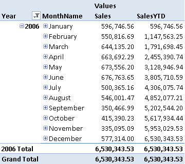
You can see the result of Sales and SalesYTD in Figure 2.
You can apply the same pattern for different time intelligence calculations by modifying the logical condition of the FILTER function.
Important
If you are not using time intelligence functions, the presence of ALL ( ‘Date’ ) in the calculate filter automatically produces the same effect as a table marked as a date table in the data model. In fact, filtering in a CALCULATE function the date column used to mark a date table would implicitly add the same ALL ( ‘Date’ ) that you see explicitly defined in this pattern. However, when you implement custom time-related calculations, it is always a good practice to mark a table as a date table, even if you do not use the DAX time intelligence functions.
Use Cases
You can use the Time Intelligence pattern whenever using the standard DAX time intelligence functions is not an option (for example, if you need a custom calendar). The pattern is very flexible and moves the business logic of the time-related calculations from the DAX predefined functions to the content of the Date table. The following is a list of some interesting use cases.
Week-Based and ISO 8601 Calendars
The time intelligence functions in DAX (such as TOTALYTD, SAMEPERIODLASTYEAR, and many others) assume that every day in a month belongs to the same quarter regardless of the year. This assumption is not valid for a week-based calendar, in which each quarter and each year might contain days that are not “naturally” related. For example, in an ISO 8601 calendar, January 1 and January 2 of 2011 belong to week 52 of year 2010, and the first week of 2011 starts on January 3. This approach is common in the retail and manufacturing industries, where the 4-4-5 calendar, 5-4-4 calendar, and 4-5-4 calendar are used. By using 4-4-5 weeks in a quarter, you can easily compare uniform numbers between quar-ters, mainly because you have the same number of working days and weekends in each quarter. You can find further information about these calendars on Wikipedia (see the 4-4-5 calendar and ISO week date pages). The Time Intelligence pattern can handle any type of custom calendar. You can find also a specific implementation of week-based calendar pattern in the Week-Based Time Intelligence in DAX article published on SQLBI.
DirectQuery
When you use the DirectQuery feature in an Analysis Services Tabular model, DAX queries are converted into SQL code sent to the underlying SQL Server data source, but the DAX time intelligence functions are not available. You can use the Time Intelligence pattern to implement time-related calculations using DirectQuery.
Complete Pattern
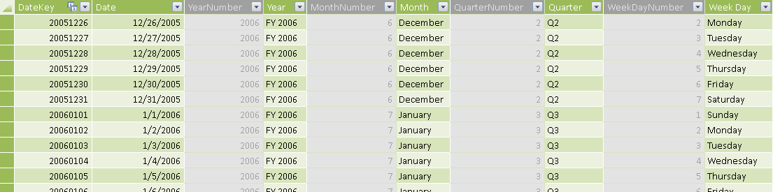
The Date table must contain all the attributes used in the calculation, in a numeric format. For example, the fiscal calendar shown in Figure 3 has strings for visible columns (Year, Month, Quarter, and Week Day), along with corresponding numeric values in other columns (YearNumber, MonthNumber, QuarterNumber, and WeekDayNumber). You will hide the numeric values from client tools in the data model but use them to implement time intelligence calculations in DAX and to sort the string columns.
In order to support comparison between periods and other calculations, the Date table also contains:
- A sequential number of days within the current year, quarter, and month.
- A sequential number of quarters and months elapsed since a reference date (which could be the beginning of the calendar).
- The total number of days in the current quarter and month.
These additional columns are visible in Figure 4.

Aggregation Pattern
Any aggregation over time filters the Date table to include all the dates in the period considered. The only difference in each formula is the condition that checks whether the date belongs to the considered aggregation or not.
The general formula will be:
[AggregationOverTime] :=
CALCULATE (
    [OriginalMeasure],
    FILTER (
        ALL ( 'Date' ),
        <check whether the date belongs to the aggregation>
    )
)
When you define an aggregation, usually you extend the period considered to include all the days elapsed since a particular day in the past. However, it is best to not make any assumption about the calendar structure, instead writing a condition that entirely depends on the data in the table. For example, you can write the year-to-date in this way:
[YTD] :=
CALCULATE (
    [OriginalMeasure],
    FILTER (
        ALL ( 'Date' ),
        'Date'[Year] = MAX ( 'Date'[Year] )
            && 'Date'[Date] <= MAX ( 'Date'[Date] )
    )
)
However, a calculation of the last 12 months would be more complicated, because there could be leap years (with February having 29 days instead of 28) and the year might not start on January 1. A calculated column can have information that simplifies the condition. For example, the SequentialDayNumber column contains the running total of days in the Date table, excluding February 29. This is the formula used to define such a calculated column:
= COUNTROWS (
    FILTER (
        ALL ( Date ),
        'Date'[Date] <= EARLIER ( 'Date'[Date] )
            && NOT ( MONTH ( 'Date'[Date] ) = 2 && DAY ( 'Date'[Date] ) = 29 )
    )
)
When the formula is written in this way, February 29 will have always the same SequentialDayNumber as February 28. You can write the moving annual total (the total of the last 12 months) as the total of the last 365 days. Since the test is based on SequentialDayNumber, February 29 will be automatically included in the range, which will consider 366 days instead of 365.
[MAT Sales] :=
CALCULATE (
    [Sales],
    FILTER (
        ALL ( 'Date' ),
        'Date'[SequentialDayNumber] > MAX ( 'Date'[SequentialDayNumber] ) - 365
             && 'Date'[SequentialDayNumber] <= MAX ( 'Date'[SequentialDayNumber] )
    )
)
A complete list of calculations is included in the More Patterns section.
Period Comparison Pattern
You can write the calculation for an aggregation by simply using the date, even if the SequentialDayNumber column is required to handle leap years. The period comparison can be more complex, because it requires detection of the current selection in order to apply the correct filter on dates to get a parallel period. For example, to calculate the year-over-year difference, you need the value of the same selection in the previous year. This analysis complicates the DAX formula required, but it is necessary if you want a behavior similar to the DAX time intelligence functions for your custom calendar.
The following implementation assumes that the calendar month drives the logic to select a corresponding comparison period. If the user selects all the days in a month, that entire month will be selected in a related period (a month, quarter, or year back in time) for the comparison. If instead she selects only a few days in a month, then only the corresponding days in the same month will be selected in the related period. You can implement a different logic (based on weeks, for example) by changing the filter expression that selects the days to compare with.
For example, the month-over-month calculation (MOM) compares the current selection with the same selection one month before.
[MOM Sales] := [Sales] – [PM Sales]

[MOM% Sales] := DIVIDE ( [MOM Sales], [PM Sales] )
The complex part is the calculation of the corresponding selection for the previous month (PM Sales). The formula iterates the YearMonthNumber column, which contains a unique value for each month and year.
SUMX (
    VALUES ( 'Date'[YearMonthNumber] ),
    <calculation for the month>
)
The calculation is different depending on whether all the days of the month are included in the selection or not. So the first part of the calculation performs this check.
    IF (
        CALCULATE ( COUNTROWS ( VALUES ( 'Date'[Date] ) ) )
            = CALCULATE ( VALUES ( 'Date'[MonthDays] ) ),
        <calculation for all days selected in the month>,
        <calculation for partial selection of the days in the month>
    )
If the number of days selected is equal to the number of days in the month (stored in the MonthDays column), then the filter selects all the days in the previous month (by subtracting one from the YearMonthNumber column).
        CALCULATE (
            [Sales],
            ALL ( 'Date' ),
            FILTER (
                ALL ( 'Date'[YearMonthNumber] ),
                'Date'[YearMonthNumber]
                    = EARLIER ( 'Date'[YearMonthNumber] ) - 1
            )
        )
Otherwise, the filter also includes the days selected in the month iterated (MonthDayNumber column); such a filter is highlighted in the following formula.
        CALCULATE (
            [Sales],
            ALL ( 'Date' ),
            CALCULATETABLE ( VALUES ( 'Date'[MonthDayNumber] ) ),
            FILTER (
                ALL ( 'Date'[YearMonthNumber] ),
                'Date'[YearMonthNumber]
                    = EARLIER ( 'Date'[YearMonthNumber] ) - 1
            )
        )
    )
The complete formula for the sales in the previous month is as follows.
[PM Sales] :=
SUMX (
    VALUES ( 'Date'[YearMonthNumber] ),
    IF (
        CALCULATE ( COUNTROWS ( VALUES ( 'Date'[Date] ) ) )
            = CALCULATE ( VALUES ( 'Date'[MonthDays] ) ),
        CALCULATE (
            [Sales],
            ALL ( 'Date' ),
            FILTER (
                ALL ( 'Date'[YearMonthNumber] ),
                'Date'[YearMonthNumber]
                    = EARLIER ( 'Date'[YearMonthNumber] ) - 1
            )
        ),
        CALCULATE (
            [Sales],
            ALL ( 'Date' ),
            CALCULATETABLE ( VALUES ( 'Date'[MonthDayNumber] ) ),
            FILTER (
                ALL ( 'Date'[YearMonthNumber] ),
                'Date'[YearMonthNumber]
                    = EARLIER ( 'Date'[YearMonthNumber] ) - 1
            )
        )
    )
)
The other calculations for previous quarter and previous year simply change the number of months subtracted in the filter on YearMonthNumber column. The complete formulas are included in the More Pattern Examples section.
Semi-Additive Pattern
Semi-additive measures require a particular calculation when you compare data over different periods. The simple calculation requires the LASTDATE function, which you can use also with custom calendars:
[Balance] :=
CALCULATE (
    [Inventory Value],
    LASTDATE ( 'Date'[Date] )
)
However, if you want to avoid any time intelligence calculation due to incompatibility with DirectQuery mode, you can use the following syntax:
[Balance DirectQuery] :=
CALCULATE (
    [Inventory Value],
    FILTER (
        'Date'[Date],
        'Date'[Date] = MAX ( 'Date'[Date] )
    )
)
You do not need to compute aggregations over time for semi-additive measures because of their nature: you need only the last day of the period and you can ignore values in other days. However, a different calculation is required if you want to compare a semi-additive measure over different periods. For example, if you want to compare the last day in two different month-based periods, you need a more complex logic to identify the last day because the months may have different lengths. A simple solution is to create a calculated column for each offset you want to handle, directly storing the corresponding date in the previous month, quarter, or year. For example, you can obtain the corresponding “last date” in the previous month with this calculated column:
'Date'[PM Date] =
CALCULATE (
    MAX  ( 'Date'[Date] ),
    ALL ( 'Date' ),
    FILTER (
        ALL ( 'Date'[MonthDayNumber] ),
        'Date'[MonthDayNumber] <= EARLIER ( 'Date'[MonthDayNumber] )
            || EARLIER ( 'Date'[MonthDayNumber] ) = EARLIER ( 'Date'[MonthDays] )
    ),
    FILTER (
        ALL ( 'Date'[YearMonthNumber] ),
        'Date'[YearMonthNumber]
            = EARLIER ( 'Date'[YearMonthNumber] ) – 1
    )
)
The logic behind the formula is that you consider the last available date in the previous month, so that if it has fewer days than the current month, you get the last available one. For example, for March 30, you will get February 28 or 29. However, if the previous month has more days than the current month, you still get the last day available, thanks to the condition that does not filter any MonthDayNumber if it is equal to MonthDays, which is the number of days in the current month. For example, for September 30, you will obtain August 31 as a result. You will just change the comparison to YearMonthNumber if you want to get the previous quarter or year, using 3 or 12, respectively, instead of 1 in this filter of [PQ Date] and [PY Date] calculated columns:
'Date'[PQ Date] =
...
        'Date'[YearMonthNumber]
            = EARLIER ( 'Date'[YearMonthNumber] ) – 3
...
'Date'[PY Date] =
...
        'Date'[YearMonthNumber]
            = EARLIER ( 'Date'[YearMonthNumber] ) – 12
...
Having an easy way to get the corresponding last date of the previous month, you can now write a short definition of the previous month Balance measure, by just using MAX ( Date[PM Date] ) to filter the date:
[PM Balance] :=
CALCULATE (
    Inventory[Inventory Value],
    FILTER (
        ALL ( 'Date' ),
        'Date'[Date] = MAX ( 'Date'[PM Date] )
    )
)
You can define the measures for the previous quarter and previous year just by changing the measure used in the MAX function, using [PQ Date] and [PY Date], respectively. These columns are useful also for implementing the comparison of aggregations over periods, such as Month Over Month To Date, as shown in the More Pattern Examples section.
More Pattern Examples
This section shows the time patterns for different types of calculations that you can apply to a custom monthly-based calendar without relying on DAX time intelligence functions. The measures defined will use the following naming convention:
| Acronym | Description | Shift Period | Aggregation | Comparison |
|---|---|---|---|---|
| YTD | Year To Date |
X |
||
| QTD | Quarter To Date |
X |
||
| MTD | Month To Date |
X |
||
| MAT | Moving Annual Total |
X |
||
| PY | Previous Year |
X |
||
| PQ | Previous Quarter |
X |
||
| PM | Previous Month |
X |
||
| PP | Previous Period (automatically selects year, quarter, or month) |
X |
||
| PMAT | Previous Year Moving Annual Total |
X |
X |
|
| YOY | Year Over Year |
X |
||
| QOQ | Quarter Over Quarter |
X |
||
| MOM | Month Over Month |
X |
||
| POP | Period Over Period (automatically selects year, quarter, or month) |
X |
||
| AOA | Moving Annual Total Over Moving Annual Total |
X |
X |
|
| PYTD | Previous Year To Date |
X |
X |
|
| PQTD | Previous Quarter To Date |
X |
X |
|
| PMTD | Previous Month To Date |
X |
X |
|
| YOYTD | Year Over Year To Date |
X |
X |
X |
| QOQTD | Quarter Over Quarter To Date |
X |
X |
X |
| MOMTD | Month Over Month To Date |
X |
X |
X |
Complete Period Comparison Patterns
The formulas in this section define the different aggregations over time.
Additive Measures
[PY Sales] :=
SUMX (
    VALUES ( 'Date'[YearMonthNumber] ),
    IF (
        CALCULATE (
            COUNTROWS (
                VALUES ( 'Date'[Date] )
            )
        )
            = CALCULATE (
                VALUES ( 'Date'[MonthDays] )
            ),
        CALCULATE (
            [Sales],
            ALL ( 'Date' ),
            FILTER (
                ALL ( 'Date'[YearMonthNumber] ),
                'Date'[YearMonthNumber]
                    = EARLIER ( 'Date'[YearMonthNumber] ) – 12
            )
        ),
        CALCULATE (
            [Sales],
            ALL ( 'Date' ),
            CALCULATETABLE (
                VALUES ( 'Date'[MonthDayNumber] )
            ),
            FILTER (
                ALL ( 'Date'[YearMonthNumber] ),
                'Date'[YearMonthNumber]
                    = EARLIER ( 'Date'[YearMonthNumber] ) – 12
            )
        )
    )
)
[PQ Sales] :=
SUMX (
    VALUES ( 'Date'[YearMonthNumber] ),
    IF (
        CALCULATE (
            COUNTROWS (
                VALUES ( 'Date'[Date] )
            )
        )
            = CALCULATE (
                VALUES ( 'Date'[MonthDays] )
            ),
        CALCULATE (
            [Sales],
            ALL ( 'Date' ),
            FILTER (
                ALL ( 'Date'[YearMonthNumber] ),
                'Date'[YearMonthNumber]
                    = EARLIER ( 'Date'[YearMonthNumber] ) – 3
            )
        ),
        CALCULATE (
            [Sales],
            ALL ( 'Date' ),
            CALCULATETABLE (
                VALUES ( 'Date'[MonthDayNumber] )
            ),
            FILTER (
                ALL ( 'Date'[YearMonthNumber] ),
                'Date'[YearMonthNumber]
                    = EARLIER ( 'Date'[YearMonthNumber] ) – 3
            )
        )
    )
)
[PM Sales] :=
SUMX (
    VALUES ( 'Date'[YearMonthNumber] ),
    IF (
        CALCULATE (
            COUNTROWS (
                VALUES ( 'Date'[Date] )
            )
        )
            = CALCULATE (
                VALUES ( 'Date'[MonthDays] )
            ),
        CALCULATE (
            [Sales],
            ALL ( 'Date' ),
            FILTER (
                ALL ( 'Date'[YearMonthNumber] ),
                'Date'[YearMonthNumber]
                    = EARLIER ( 'Date'[YearMonthNumber] ) – 1
            )
        ),
        CALCULATE (
            [Sales],
            ALL ( 'Date' ),
            CALCULATETABLE (
                VALUES ( 'Date'[MonthDayNumber] )
            ),
            FILTER (
                ALL ( 'Date'[YearMonthNumber] ),
                'Date'[YearMonthNumber]
                    = EARLIER ( 'Date'[YearMonthNumber] ) – 1
            )
        )
    )
)
[PP Sales] :=
SWITCH (
    TRUE,
    ISFILTERED ( 'Date'[Month] ), [PM Sales],
    ISFILTERED ( 'Date'[Quarter] ), [PQ Sales],
    ISFILTERED ( 'Date'[Year] ), [PY Sales],
    BLANK ()
)
[YOY Sales] :=
[Sales] - [PY Sales]
[QOQ Sales] :=
[Sales] - [PQ Sales]
[MOM Sales] :=
[Sales] - [PM Sales]
[POP Sales] :=
[Sales] - [PP Sales]
[YOY% Sales] :=
DIVIDE ( [YOY Sales], [PY Sales] )
[QOQ% Sales] :=
DIVIDE ( [QOQ Sales], [PQ Sales] )
[MOM% Sales] :=
DIVIDE ( [MOM Sales], [PM Sales] )
[POP% Sales] :=
DIVIDE ( [POP Sales], [PP Sales] )
Semi-Additive Measures
[Balance] :=
CALCULATE (
    Inventory[Inventory Value],
    FILTER (
        ALL ( 'Date'[Date] ),
        'Date'[Date] = MAX ( 'Date'[Date] )
    )
)
[PY Balance] :=
CALCULATE (
    Inventory[Inventory Value],
    FILTER (
        ALL ( 'Date' ),
        'Date'[Date] = MAX ( 'Date'[PY Date] )
    )
)
[PQ Balance] :=
CALCULATE (
    Inventory[Inventory Value],
    FILTER (
        ALL ( 'Date' ),
        'Date'[Date] = MAX ( 'Date'[PQ Date] )
    )
)
[PM Balance] :=
CALCULATE (
    Inventory[Inventory Value],
    FILTER (
        ALL ( 'Date' ),
        'Date'[Date] = MAX ( 'Date'[PM Date] )
    )
)
[PP Balance] :=
CALCULATE (
    Inventory[Inventory Value],
    FILTER (
        ALL ( 'Date' ),
        'Date'[Date] = MAX ( 'Date'[PP Date] )
    )
)
[YOY Balance] :=
[Balance] - [PY Balance]
[QOQ Balance] :=
[Balance] - [PQ Balance]
[MOM Balance] :=
[Balance] - [PM Balance]
[POP Balance] :=
[Balance] - [PP Balance]
[YOY% Balance] :=
DIVIDE ( [YOY Balance], [PY Balance] )
[QOQ% Balance] :=
DIVIDE ( [QOQ Balance], [PQ Balance] )
[MOM% Balance] :=
DIVIDE ( [MOM Balance], [PM Balance] )
[POP% Balance] :=
DIVIDE ( [POP Balance], [PP Balance] )
Complete Aggregation Patterns
The formulas in this section define the different aggregations over time.
Simple Aggregation for Additive Measures
[Sales] :=
SUM ( Sales[SalesAmount] )
[YTD Sales] :=
CALCULATE (
    [Sales],
    FILTER (
        ALL ( DATE ),
        'Date'[YearNumber] = MAX ( 'Date'[YearNumber] )
            && 'Date'[Date] <= MAX ( 'Date'[Date] )
    )
)
[QTD Sales] :=
CALCULATE (
    [Sales],
    FILTER (
        ALL ( DATE ),
        'Date'[YearQuarterNumber] = MAX ( 'Date'[YearQuarterNumber] )
            && 'Date'[Date] <= MAX ( 'Date'[Date] )
    )
)
[MTD Sales] :=
CALCULATE (
    [Sales],
    FILTER (
        ALL ( DATE ),
        'Date'[YearMonthNumber] = MAX ( 'Date'[YearMonthNumber] )
            && 'Date'[Date] <= MAX ( 'Date'[Date] )
    )
)
[MAT Sales] :=
CALCULATE (
    [Sales],
    FILTER (
        ALL ( 'Date' ),
        'Date'[SequentialDayNumber] > MAX ( 'Date'[SequentialDayNumber] ) - 365
             && 'Date'[SequentialDayNumber] <= MAX ( 'Date'[SequentialDayNumber] )
    )
)
Combined Aggregation and Period Comparison for Additive Measures
The measures that combine aggregation and period comparison are implemented using the calculated columns (in the Date table) that return the corresponding date in a previous period (year, quarter, and month).
[PYTD Sales] :=
CALCULATE (
    [Sales],
    FILTER (
        ALL ( DATE ),
        'Date'[YearNumber] = MAX ( 'Date'[YearNumber] ) – 1
            && 'Date'[Date] <= MAX ( 'Date'[PY Date] )
    )
)
[PQTD Sales] :=
CALCULATE (
    [Sales],
    FILTER (
        ALL ( DATE ),
        'Date'[YearQuarterNumber] = MAX ( 'Date'[YearQuarterNumber] ) – 1
            && 'Date'[Date] <= MAX ( 'Date'[PQ Date] )
    )
)
[PMTD Sales] :=
CALCULATE (
    [Sales],
    FILTER (
        ALL ( DATE ),
        'Date'[YearMonthNumber] = MAX ( 'Date'[YearMonthNumber] ) – 1
            && 'Date'[Date] <= MAX ( 'Date'[PM Date] )
    )
)
[PMAT Sales] :=
CALCULATE (
    [Sales],
    FILTER (
        ALL ( 'Date' ),
        'Date'[SequentialDayNumber] > MAX ( 'Date'[SequentialDayNumber] ) – 730
             && 'Date'[SequentialDayNumber] <= MAX ( 'Date'[SequentialDayNumber] ) – 365
    )
)
[YOYTD Sales] :=
[YTD Sales] - [PYTD Sales]
[QOQTD Sales] :=
[QTD Sales] - [PQTD Sales]
[MOMTD Sales] :=
[MTD Sales] - [PMTD Sales]
[AOA Sales] :=
[MAT Sales] - [PMAT Sales]
[YOYTD% Sales] :=
DIVIDE ( [YOYTD Sales], [PYTD Sales] )
[QOQTD% Sales] :=
DIVIDE ( [QOQTD Sales], [PQTD Sales] )
[MOMTD% Sales] :=
DIVIDE ( [MOMTD Sales], [PMTD Sales] )
[AOA% Sales] :=
DIVIDE ( [AOA Sales], [PMAT Sales] )
Evaluates an expression in a context modified by filters.
CALCULATE ( <Expression> [, <Filter> [, <Filter> [, … ] ] ] )
Returns a table that has been filtered.
FILTER ( <Table>, <FilterExpression> )
Returns all the rows in a table, or all the values in a column, ignoring any filters that might have been applied.
ALL ( [<TableNameOrColumnName>] [, <ColumnName> [, <ColumnName> [, … ] ] ] )
Evaluates the specified expression over the interval which begins on the first day of the year and ends with the last date in the specified date column (or in the evaluation context if a calendar reference is provided) after applying specified filters.
TOTALYTD ( <Expression>, <Dates> [, <Filter>] [, <YearEndDate>] )
Returns a set of dates in the current selection from the previous year.
SAMEPERIODLASTYEAR ( <Dates> )
Returns last non blank date.
LASTDATE ( <Dates> )
Returns the largest value in a column, or the larger value between two scalar expressions. Ignores logical values. Strings are compared according to alphabetical order.
MAX ( <ColumnNameOrScalar1> [, <Scalar2>] )
This pattern is designed for Excel 2010-2013. An alternative version for Power BI / Excel 2016-2019 is also available.
This pattern is included in the book DAX Patterns 2015.


Downloads
Download the sample files for Excel 2010-2013: