IMPORTANT
If you use Power BI, Analysis Services, or Excel 2016 or later versions, you can use the statistical functions in DAX.
If you use Excel 2010 or Excel 2013, most of the DAX statistical functions are not available and you can rely on an alternative implementation based on DAX code as described in this page.

DAX includes a few statistical aggregation functions, such as average, variance, and standard deviation. Other typical statistical calculations require you to write longer DAX expressions. Excel, from this point of view, has a much richer language.

The Statistical Patterns are a collection of common statistical calculations: median, mode, moving average, percentile, and quartile. We would like to thank Colin Banfield, Gerard Brueckl, and Javier Guillén, whose blogs inspired some of the following patterns.

Basic Pattern Example

The formulas in this pattern are the solutions to specific statistical calculations.

Average

You can use standard DAX functions to calculate the mean (arithmetic average) of a set of values.

AVERAGE: returns the average of all the numbers in a numeric column.
AVERAGEA: returns the average of all the numbers in a column, handling both text and non-numeric values (non-numeric and empty text values count as 0).
AVERAGEX: calculate the average on an expression evaluated over a table.

Moving Average

The moving average is a calculation to analyze data points by creating a series of averages of different subsets of the full data set. You can use many DAX techniques to implement this calculation. The simplest technique is using AVERAGEX, iterating a table of the desired granularity and calculating for each iteration the expression that generates the single data point to use in the average. For example, the following formula calculates the moving average of the last 7 days, assuming that you are using a Date table in your data model.

Moving AverageX 7 Days :=
AVERAGEX (
    DATESINPERIOD (
        'Date'[Date],
        LASTDATE ( 'Date'[Date] ),
        -7,
        DAY
    ),
    [Total Amount]
)

Using AVERAGEX, you automatically calculate the measure at each granularity level. When using a measure that can be aggregated (such as SUM), then another approach—based on CALCULATE—may be faster. You can find this alternative approach in the complete pattern of Moving Average.

Variance

You can use standard DAX functions to calculate the variance of a set of values.

VAR.S: returns the variance of values in a column representing a sample population.
VAR.P: returns the variance of values in a column representing the entire population.
VARX.S: returns the variance of an expression evaluated over a table representing a sample population.
VARX.P: returns the variance of an expression evaluated over a table representing the entire population.

Standard Deviation

You can use standard DAX functions to calculate the standard deviation of a set of values.

STDEV.S: returns the standard deviation of values in a column representing a sample population.
STDEV.P: returns the standard deviation of values in a column representing the entire population.
STDEVX.S: returns the standard deviation of an expression evaluated over a table representing a sample population.
STDEVX.P: returns the standard deviation of an expression evaluated over a table representing the entire population.

Median

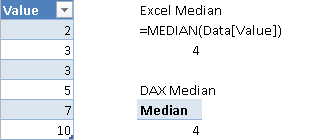
The median is the numerical value separating the higher half of a population from the lower half. If there is an odd number of rows, the median is the middle value (sorting the rows from the lowest value to the highest value). If there is an even number of rows, it is the average of the two middle values. The formula ignores blank values, which are not considered part of the population. The result is identical to the MEDIAN function in Excel.

Median :=
(
    MINX (
        FILTER (
            VALUES ( Data[Value] ),
            CALCULATE (
                COUNT ( Data[Value] ),
                Data[Value]
                    <= EARLIER ( Data[Value] )
            )
                > COUNT ( Data[Value] ) / 2
        ),
        Data[Value]
    )
        + MINX (
            FILTER (
                VALUES ( Data[Value] ),
                CALCULATE (
                    COUNT ( Data[Value] ),
                    Data[Value]
                        <= EARLIER ( Data[Value] )
                )
                    > ( COUNT ( Data[Value] ) - 1 ) / 2
            ),
            Data[Value]
        )
) / 2

Figure 1 shows a comparison between the result returned by Excel and the corresponding DAX formula for the median calculation.

Mode

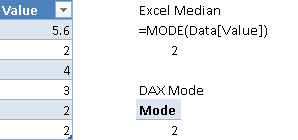
The mode is the value that appears most often in a set of data. The formula ignores blank values, which are not considered part of the population. The result is identical to the MODE and MODE.SNGL functions in Excel, which return only the minimum value when there are multiple modes in the set of values considered. The Excel function MODE.MULT would return all of the modes, but you cannot implement it as a measure in DAX.

Mode :=
MINX (
    TOPN (
        1,
        ADDCOLUMNS (
            VALUES ( Data[Value] ),
            "Frequency", CALCULATE ( COUNT ( Data[Value] ) )
        ),
        [Frequency],
        0
    ),
    Data[Value]
)

Figure 2 compares the result returned by Excel with the corresponding DAX formula for the mode calculation.

Percentile

The percentile is the value below which a given percentage of values in a group falls. The formula ignores blank values, which are not considered part of the population. The calculation in DAX requires several steps, described in the Complete Pattern section, which shows how to obtain the same results of the Excel functions PERCENTILE, PERCENTILE.INC, and PERCENTILE.EXC.

Quartile

The quartiles are three points that divide a set of values into four equal groups, each group comprising a quarter of the data. You can calculate the quartiles using the Percentile pattern, following these correspondences:

First quartile = lower quartile = 25^th percentile
Second quartile = median = 50^th percentile
Third quartile = upper quartile = 75^th percentile

Complete Pattern

A few statistical calculations have a longer description of the complete pattern, because you might have different implementations depending on data models and other requirements.

Moving Average

Usually you evaluate the moving average by referencing the day granularity level. The general template of the following formula has these markers:

<number_of_days> is the number of days for the moving average.
<date_column> is the date column of the date table if you have one, or the date column of the table containing values if there is no separate date table.
<measure> is the measure to compute as the moving average.

The simplest pattern uses the AVERAGEX function in DAX, which automatically considers only the days for which there is a value.

Moving AverageX <number_of_days> Days:=
AVERAGEX (
    FILTER (
        ALL ( <date_column> ),
        <date_column> > ( MAX ( <date_column> ) - <number_of_days> )
            && <date_column> <= MAX ( <date_column> )
    ),
    <measure>
)

As an alternative, you can use the following template in data models without a date table and with a measure that can be aggregated (such as SUM) over the entire period considered.

Moving Average <number_of_days> Days:=
CALCULATE (
    IF (
        COUNT ( <date_column> ) >= <number_of_days>,
        SUM ( Sales[Amount] ) / COUNT ( <date_column> )
    ),
    FILTER (
        ALL ( <date_column> ),
        <date_column> > ( MAX ( <date_column> ) - <number_of_days> )
            && <date_column> <= MAX ( <date_column> )
    )
)

The previous formula considers a day with no corresponding data as a measure that has 0 value. This can happen only when you have a separate date table, which might contain days for which there are no corresponding transactions. You can fix the denominator for the average using only the number of days for which there are transactions using the following pattern, where:

<fact_table> is the table related to the date table and containing values computed by the measure.

Moving Average <number_of_days> Days No Zero:=
CALCULATE (
    IF (
        COUNT ( <date_column> ) >= <number_of_days>,
        SUM ( Sales[Amount] ) / CALCULATE ( COUNT ( <date_column> ), <fact_table> )
    ),
    FILTER (
        ALL ( <date_column> ),
        <date_column> > ( MAX ( <date_column> ) - <number_of_days> )
            && <date_column> <= MAX ( <date_column> )
    )
)

You might use the DATESBETWEEN or DATESINPERIOD functions instead of FILTER, but these work only in a regular date table, whereas you can apply the pattern described above also to non-regular date tables and to models that do not have a date table.

For example, consider the different results produced by the following two measures.

Moving Average 7 Days :=
CALCULATE (
    IF (
        COUNT ( 'Date'[Date] ) >= 7,
        SUM ( Sales[Amount] ) / COUNT ( 'Date'[Date] )
    ),
    FILTER (
        ALL ( 'Date'[Date] ),
        'Date'[Date] > ( MAX ( 'Date'[Date] ) - 7 )
            && 'Date'[Date] <= MAX ( 'Date'[Date] )     ) )

Moving Average 7 Days No Zero :=
CALCULATE (
    IF (
        COUNT ( 'Date'[Date] ) >= 7,
        SUM ( Sales[Amount] ) / CALCULATE ( COUNT ( 'Date'[Date] ), Sales )
    ),
    FILTER ( 
        ALL ( 'Date'[Date] ),
        'Date'[Date] > ( MAX ( 'Date'[Date] ) - 7 )
            && 'Date'[Date] <= MAX ( 'Date'[Date] )
    )
)

In Figure 3, you can see that there are no sales on September 11, 2005. However, this date is included in the Date table; thus, there are 7 days (from September 11 to September 17) that have only 6 days with data.

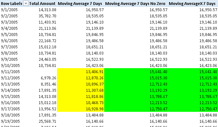
The measure Moving Average 7 Days has a lower number between September 11 and September 17, because it considers September 11 as a day with 0 sales. If you want to ignore days with no sales, then use the measure Moving Average 7 Days No Zero. This could be the right approach when you have a complete date table but you want to ignore days with no transactions. Using the Moving Average 7 Days formula, the result is correct because AVERAGEX automatically considers only non-blank values.

Keep in mind that you might improve the performance of a moving average by persisting the value in a calculated column of a table with the desired granularity, such as date, or date and product. However, the dynamic calculation approach with a measure offers the ability to use a parameter for the number of days of the moving average (e.g., replace <number_of_days> with a measure implementing the Parameters Table pattern).

Median

The median corresponds to the 50^th percentile, which you can calculate using the Percentile pattern. However, the Median pattern allows you to optimize and simplify the median calculation using a single measure, instead of the several measures required by the Percentile pattern. You can use this approach when you calculate the median for values included in <value_column>, as shown below:

Median :=
(
    MINX (
        FILTER (
            VALUES ( <value_column> ),
            CALCULATE (
                COUNT ( <value_column> ),
                <value_column>
                    <= EARLIER ( <value_column> )
            )
                > COUNT ( <value_column> ) / 2
        ),
        <value_column>
    )
        + MINX (
            FILTER (
                VALUES ( <value_column> ),
                CALCULATE (
                    COUNT ( <value_column> ),
                    <value_column>
                        <= EARLIER ( <value_column> )
                )
                    > ( COUNT ( <value_column> ) - 1 ) / 2
            ),
            <value_column>
        )
) / 2

To improve performance, you might want to persist the value of a measure in a calculated column, if you want to obtain the median for the results of a measure in the data model. However, before doing this optimization, you should implement the MedianX calculation based on the following template, using these markers:

<granularity_table> is the table that defines the granularity of the calculation. For example, it could be the Date table if you want to calculate the median of a measure calculated at the day level, or it could be VALUES ( ‘Date'[YearMonth] ) if you want to calculate the median of a measure calculated at the month level.
<measure> is the measure to compute for each row of <granularity_table> for the median calculation.
<measure_table> is the table containing data used by <measure>. For example, if the <granularity_table> is a dimension such as ‘Date’, then the <measure_table> will be ‘Internet Sales’ containing the Internet Sales Amount column summed by the Internet Total Sales measure.

MedianX :=
(
    MINX (
        TOPN (
            COUNTROWS ( CALCULATETABLE ( <granularity_table>, <measure_table> ) ) / 2,
            CALCULATETABLE ( <granularity_table>, <measure_table> ),
            <measure>,
            0
        ),
        <measure>
    )
        + MINX (
            TOPN (
                ( COUNTROWS ( CALCULATETABLE ( <granularity_table>, <measure_table> ) ) + 1 
                ) / 2,
                CALCULATETABLE ( <granularity_table>, <measure_table> ),
                <measure>,
                0
            ),
            <measure>
        )
) / 2

For example, you can write the median of Internet Total Sales for all the Customers in Adventure Works as follows:

MedianX :=
(
    MINX (
        TOPN (
            COUNTROWS ( CALCULATETABLE ( Customer, 'Internet Sales' ) ) / 2,
            CALCULATETABLE ( Customer, 'Internet Sales' ),
            [Internet Total Sales],
            0
        ),
        [Internet Total Sales]
    )
        + MINX (
            TOPN (
                ( COUNTROWS ( CALCULATETABLE ( Customer, 'Internet Sales' ) ) + 1 ) / 2,
                CALCULATETABLE ( Customer, 'Internet Sales' ),
                [Internet Total Sales],
                0
            ),
            [Internet Total Sales]
        )
) / 2

Tip The following pattern:
CALCULATETABLE ( <granularity_table>, <measure_table> ) 
is used to remove rows from <granularity_table> that have no corresponding data in the current selection. It is a faster way than using the following expression:
FILTER ( <granularity_table>, NOT ( ISBLANK ( <measure> ) ) ) 
However, you might replace the entire CALCULATETABLE expression with just <granularity_table> if you want to consider blank values of the <measure> as 0.

The performance of the MedianX formula depends on the number of rows in the table iterated and on the complexity of the measure. If performance is bad, you might persist the <measure> result in a calculated column of the <table>, but this will remove the ability of applying filters to the median calculation at query time.

Percentile

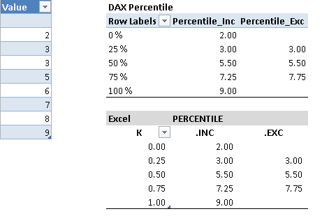
Excel has two different implementations of percentile calculation with three functions: PERCENTILE, PERCENTILE.INC, and PERCENTILE.EXC. They all return the K-th percentile of values, where K is in the range 0 to 1. The difference is that PERCENTILE and PERCENTILE.INC consider K as an inclusive range, while PERCENTILE.EXC considers the K range 0 to 1 as exclusive.

All of these functions and their DAX implementations receive a percentile value as parameter, which we call K.

<K> percentile value is in the range 0 to 1.

The two DAX implementations of percentile require a few measures that are similar, but different enough to require two different set of formulas. The measures defined in each pattern are:

K_Perc: The percentile value – it corresponds to <K>.
PercPos: The position of the percentile in the sorted set of values.
ValueLow: The value below the percentile position.
ValueHigh: The value above the percentile position.
Percentile: The final calculation of the percentile.

You need the ValueLow and ValueHigh measures in case the PercPos contains a decimal part, because then you have to interpolate between ValueLow and ValueHigh in order to return the correct percentile value.

Figure 4 shows an example of the calculations made with Excel and DAX formulas, using both algorithms of percentile (inclusive and exclusive).

In the following sections, the Percentile formulas execute the calculation on values stored in a table column, Data[Value], whereas the PercentileX formulas execute the calculation on values returned by a measure calculated at a given granularity.

Percentile Inclusive

The Percentile Inclusive implementation is the following.

K_Perc := <K>

PercPos_Inc :=
(
    CALCULATE (
        COUNT ( Data[Value] ),
        ALLSELECTED ( Data[Value] )
    ) – 1
) * [K_Perc]

ValueLow_Inc :=
MINX (
    FILTER (
        VALUES ( Data[Value] ),
        CALCULATE (
            COUNT ( Data[Value] ),
            Data[Value]
                <= EARLIER ( Data[Value] )
        )
            >= ROUNDDOWN ( [PercPos_Inc], 0 ) + 1
    ),
    Data[Value]
)

ValueHigh_Inc :=
MINX (
    FILTER (
        VALUES ( Data[Value] ),
        CALCULATE (
            COUNT ( Data[Value] ),
            Data[Value]
                <= EARLIER ( Data[Value] )
        )
            > ROUNDDOWN ( [PercPos_Inc], 0 ) + 1
    ),
    Data[Value]
)

Percentile_Inc :=
IF (
    [K_Perc] >= 0 && [K_Perc] <= 1,
    [ValueLow_Inc]
        + ( [ValueHigh_Inc] - [ValueLow_Inc] )
            * ( [PercPos_Inc] - ROUNDDOWN ( [PercPos_Inc], 0 ) )
)

Percentile Exclusive

The Percentile Exclusive implementation is the following.

K_Perc := <K>

PercPos_Exc :=
(
    CALCULATE (
        COUNT ( Data[Value] ),
        ALLSELECTED ( Data[Value] )
    ) + 1
) * [K_Perc]

ValueLow_Exc :=
MINX (
    FILTER (
        VALUES ( Data[Value] ),
        CALCULATE (
            COUNT ( Data[Value] ),
            Data[Value]
                <= EARLIER ( Data[Value] )
        )
            >= ROUNDDOWN ( [PercPos_Exc], 0 ) 
    ),
    Data[Value]
)

ValueHigh_Exc :=
MINX (
    FILTER (
        VALUES ( Data[Value] ),
        CALCULATE (
            COUNT ( Data[Value] ),
            Data[Value]
                <= EARLIER ( Data[Value] )
        )
            > ROUNDDOWN ( [PercPos_Exc], 0 ) 
    ),
    Data[Value]
)

Percentile_Exc :=
IF (
    [K_Perc] > 0 && [K_Perc] < 1,
    [ValueLow_Exc]
        + ( [ValueHigh_Exc] - [ValueLow_Exc] )
            * ( [PercPos_Exc] - ROUNDDOWN ( [PercPos_Exc], 0 ) )
)

PercentileX Inclusive

The PercentileX Inclusive implementation is based on the following template, using these markers:

<granularity_table> is the table that defines the granularity of the calculation. For example, it could be the Date table if you want to calculate the percentile of a measure at the day level, or it could be VALUES ( ‘Date'[YearMonth] ) if you want to calculate the percentile of a measure at the month level.
<measure> is the measure to compute for each row of <granularity_table> for percentile calculation.
<measure_table> is the table containing data used by <measure>. For example, if the <granularity_table> is a dimension such as ‘Date,’ then the <measure_table> will be ‘Sales’ containing the Amount column summed by the Total Amount measure.

K_Perc := <K>

PercPosX_Inc :=
(
    CALCULATE (
        COUNTROWS ( CALCULATETABLE ( <granularity_table>, <measure_table> ) ),
        ALLSELECTED ( <granularity_table> )
    ) – 1
) * [K_Perc]

ValueLowX_Inc :=
MAXX (
    TOPN (
        ROUNDDOWN ( [PercPosX_Inc], 0 ) + 1,
        CALCULATETABLE ( <granularity_table>, <measure_table> ),
        <measure>,
        1
    ),
    <measure>
)

ValueHighX_Inc :=
MAXX (
    TOPN (
        ROUNDUP ( [PercPosX_Inc], 0 ) + 1,
        CALCULATETABLE ( <granularity_table>, <measure_table> ),
        <measure>,
        1
    ),
    <measure>
)

PercentileX_Inc :=
IF (
    [K_Perc] >= 0 && [K_Perc] <= 1,
    [ValueLowX_Inc]
        + ( [ValueHighX_Inc] - [ValueLowX_Inc] )
            * ( [PercPosX_Inc] - ROUNDDOWN ( [PercPosX_Inc], 0 ) )
)

For example, you can write the PercentileX_Inc of Total Amount of Sales for all the dates in the Date table as follows:

K_Perc := <K>

PercPosX_Inc :=
(
    CALCULATE (
        COUNTROWS ( CALCULATETABLE ( 'Date', Sales ) ),
        ALLSELECTED ( 'Date' )
    ) – 1
) * [K_Perc]

ValueLowX_Inc :=
MAXX (
    TOPN (
        ROUNDDOWN ( [PercPosX_Inc], 0 ) + 1,
        CALCULATETABLE ( 'Date', Sales ),
        [Total Amount],
        1
    ),
    [Total Amount]
)

ValueHighX_Inc :=
MAXX (
    TOPN (
        ROUNDUP ( [PercPosX_Inc], 0 ) + 1,
        CALCULATETABLE ( 'Date', Sales ),
        [Total Amount],
        1
    ),
    [Total Amount]
)

PercentileX_Inc :=
IF (
    [K_Perc] >= 0 && [K_Perc] <= 1,
    [ValueLowX_Inc]
        + ( [ValueHighX_Inc] - [ValueLowX_Inc] )
            * ( [PercPosX_Inc] - ROUNDDOWN ( [PercPosX_Inc], 0 ) )
)

PercentileX Exclusive

The PercentileX Exclusive implementation is based on the following template, using the same markers used in PercentileX Inclusive:

K_Perc := <K>

PercPosX_Exc :=
(
    CALCULATE (
        COUNTROWS ( CALCULATETABLE ( <granularity_table>, <measure_table> ) ),
        ALLSELECTED ( <granularity_table> )
    ) + 1
) * [K_Perc]

ValueLowX_Exc :=
MAXX (
    TOPN (
        ROUNDDOWN ( [PercPosX_Exc], 0 ),
        CALCULATETABLE ( <granularity_table>, <measure_table> ),
        <measure>,
        1
    ),
    <measure>
)

ValueHighX_Exc :=
MAXX (
    TOPN (
        ROUNDUP ( [PercPosX_Exc], 0 ),
        CALCULATETABLE ( <granularity_table>, <measure_table> ),
        <measure>,
        1
    ),
    <measure>
)

PercentileX_Exc :=
IF (
    [K_Perc] > 0 && [K_Perc] < 1,
    [ValueLowX_Exc]
        + ( [ValueHighX_Exc] - [ValueLowX_Exc] )
            * ( [PercPosX_Exc] - ROUNDDOWN ( [PercPosX_Exc], 0 ) )
)

For example, you can write the PercentileX_Exc of Total Amount of Sales for all the dates in the Date table as follows:

K_Perc := <K>

PercPosX_Exc :=
(
    CALCULATE (
        COUNTROWS ( CALCULATETABLE ( 'Date', Sales ) ),
        ALLSELECTED ( 'Date' )
    ) + 1
) * [K_Perc]

ValueLowX_Exc :=
MAXX (
    TOPN (
        ROUNDDOWN ( [PercPosX_Exc], 0 ),
        CALCULATETABLE ( 'Date', Sales ),
        [Total Amount],
        1
    ),
    [Total Amount]
)

ValueHighX_Exc :=
MAXX (
    TOPN (
        ROUNDUP ( [PercPosX_Exc], 0 ),
        CALCULATETABLE ( 'Date', Sales ),
        [Total Amount],
        1
    ),
    [Total Amount]
)

PercentileX_Exc :=
IF (
    [K_Perc] > 0 && [K_Perc] < 1,
    [ValueLowX_Exc]
        + ( [ValueHighX_Exc] - [ValueLowX_Exc] )
            * ( [PercPosX_Exc] - ROUNDDOWN ( [PercPosX_Exc], 0 ) )
)

Basic Pattern Example

Average

Moving Average

Variance

Standard Deviation

Median

Mode

Percentile

Quartile

Complete Pattern

Moving Average

Median

Percentile

Percentile Inclusive

Percentile Exclusive

PercentileX Inclusive

PercentileX Exclusive

Downloads