The Basket analysis pattern builds on a specific application of the Survey pattern. The goal of Basket analysis is to analyze relationships between events. A typical example is to analyze which products are frequently purchased together. This means they are in the same “basket”, hence the name of this pattern.

Two products are related when they are present in the same basket. In other words, the event granularity is the purchase of a product. The basket can be the most intuitive, like a sales order; but the basket can also be a customer; In that case, products are related if they are purchased by the same customer, albeit across different orders.

Because the pattern is about checking when there is a relationship between two products, the data model contains two copies of the same table of products. The two copies are named Product and And Product. The user chooses a set of products from the Product table; the measures show how likely it is that products in the And Product table are associated to the original selection.

We included in this pattern additional association rules metrics: support, confidence, and lift. These measures make it easier to understand the results and they extract richer insights from the pattern.

Defining association rules metrics

The pattern contains several measures, which we describe in detail in this section. In order to provide the definitions, we examine the orders containing at least a product of the Cameras and camcorders category and one product of the Computers category, as shown in Figure 1.

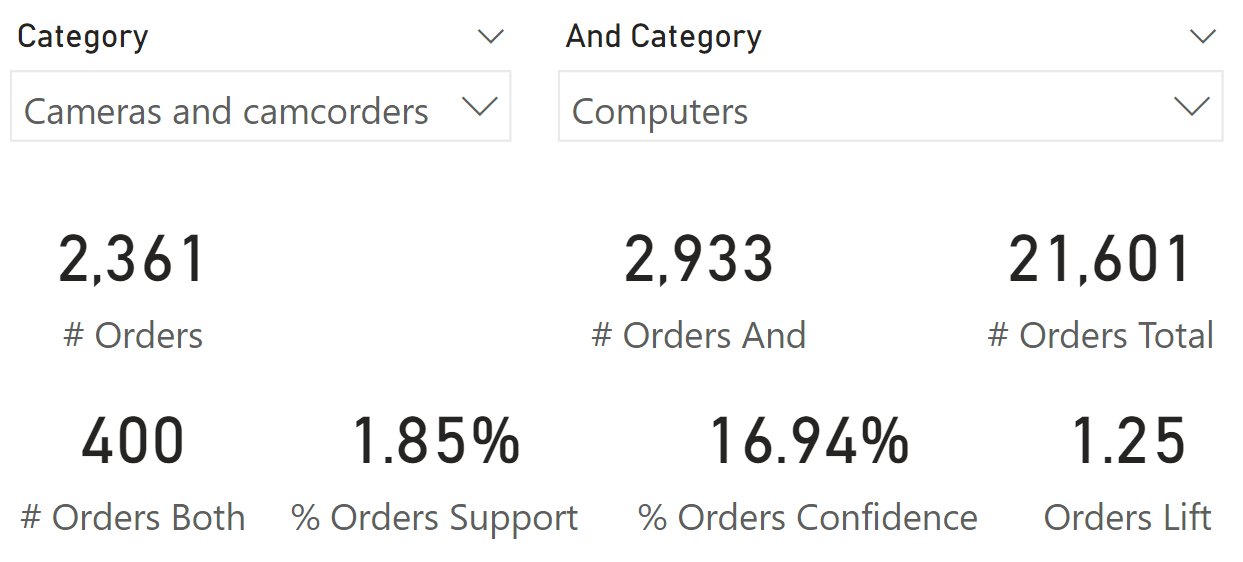
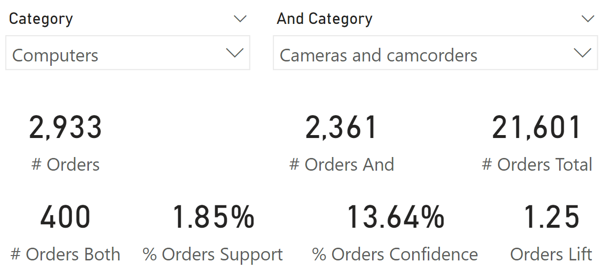
The report in Figure 1 uses two slicers: The Category slicer shows a selection of the Product[Category] column, whereas the And Category slicer shows a selection of the ‘And Product'[And Category] column. The # Orders measure shows you how many orders contain at least one product of the “Cameras and camcorders” category, whereas the # Orders And measure shows how many orders contain at least one product of both the “Cameras and camcorders” and “Computers” categories. We describe the other measures later. First, we need to make an important note: by inverting the selection between Category and And Category, the results are different by design. Most measures provide the same result (# Orders Both, % Orders Support, Orders Lift), whereas confidence (% Orders Confidence) depends on the order of the selection. In Figure 2 you can see the report from Figure 1, with the difference that the selections were inverted between the Category and And Category slicers.

Next, you find the definition of all the measures used in the pattern. There are two versions of all the measures: one considering the order as a basket, the other using the customer as a basket. For example, the description of # And applies to both # Orders And and # Customers And.

#

# Orders and # Customers return the number of unique baskets in the current filter context. Figure 1 shows 2,361 orders containing one product from the “Cameras and camcorders” category, whereas Figure 2 shows 2,933 orders containing at least one product from the “Computers” category.

# And

# Orders And and # Customers And return the number of unique baskets containing products of the And Product selection in the current filter context. These measures ignore the Product selection. Figure 1 shows 2,933 orders containing at least one product from the “Computers” category.

# Total

# Orders Total and # Customers Total return the total number of baskets and ignore any filter over Product and And Product. Both Figure 1 and Figure 2 report 21,601 orders. Be mindful that the filter on And Product is ignored by default because the relationship is not active; the only filter being explicitly ignored in the measure is the filter on Product. If there were a filter over Date, the measure would report only the baskets in the selected time period, and still ignore the filter over Product.

# Both

# Orders Both and # Customer Both return the number of unique baskets containing products from both the categories selected with the slicers. Figure 1 shows that 400 orders contain products from both categories: “Cameras and camcorders” and “Computers”.

% Support

% Orders Support and % Customers Support return the support of the association rule. Support is the ratio between # Both and # Total. Figure 1 shows that 1.85% of the orders contain products from both categories: “Cameras and camcorders” and “Computers”.

% Confidence

% Orders Confidence and % Customers Confidence return the confidence of the association rule. Confidence is the ratio between # Both and #. Figure 1 shows that out of all the orders containing “Cameras and camcorders”, 16.94% also contain “Computers” products.

Lift

Orders Lift and Customers Lift return the ratio of confidence to the probability of the selection in And Product.

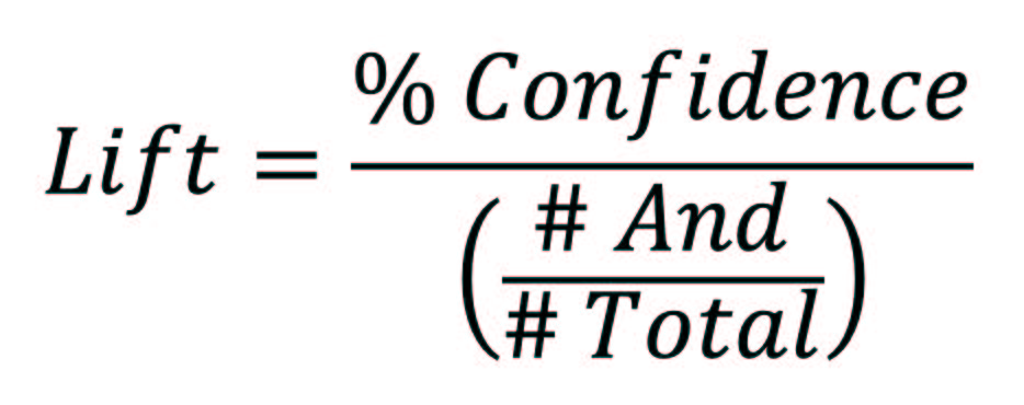
A lift greater than 1 indicates an association rule which is good enough to predict events. The greater the lift, the stronger the association. Figure 1 reports that the association rule between “Cameras and camcorders” and “Computers” is 1.25, obtained by dividing the % Confidence (16.94%) by the probability of # Orders And over # Orders Total (2933/21601 = 13.58%).

Sample reports

This section describes several reports generated on our sample model. These reports are useful to better understand the capabilities of the pattern.

The report in Figure 3 shows the products that are more likely to be present in orders containing “Contoso Optical USB Mouse M45 White”.

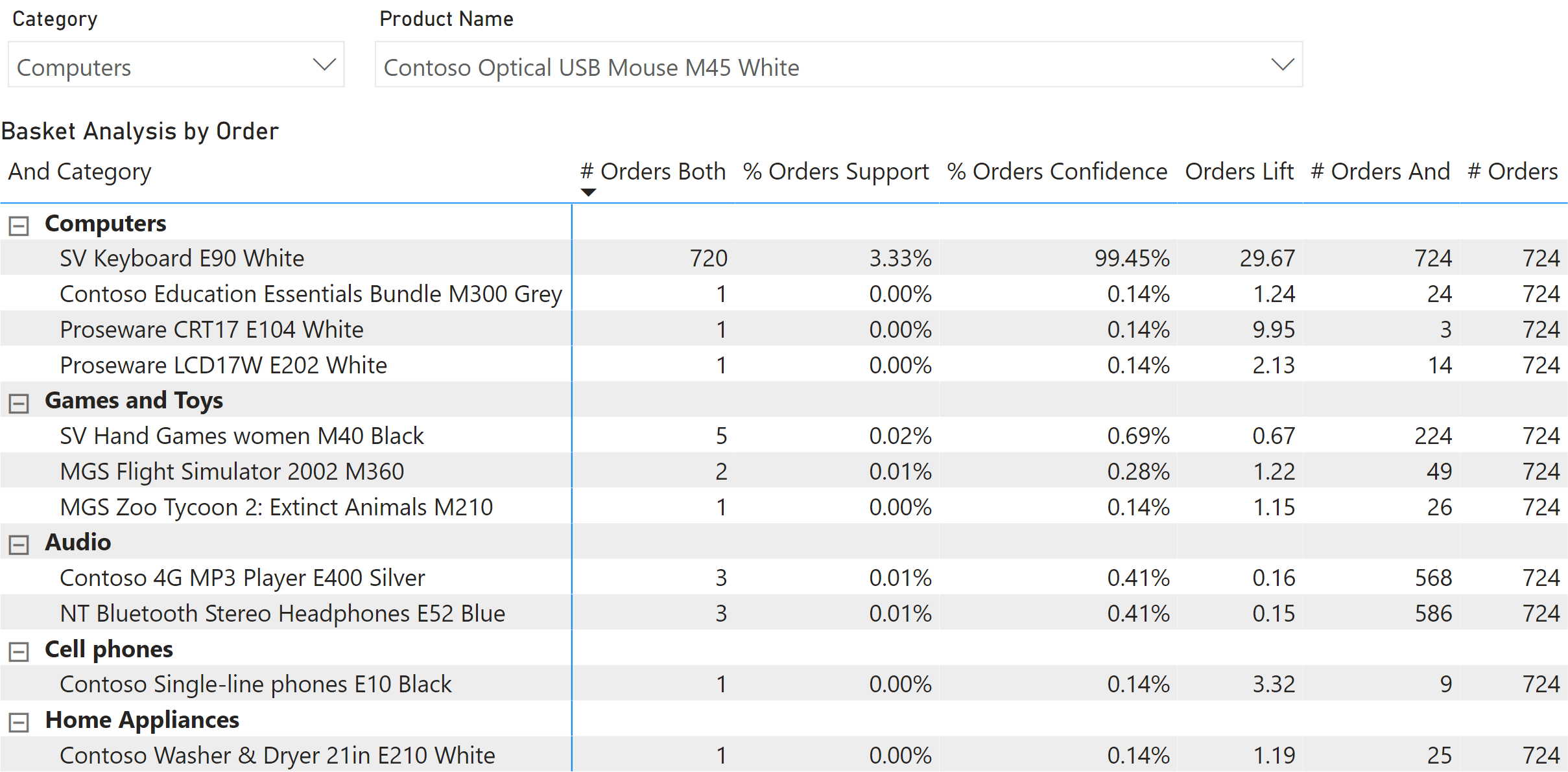
“SV Keyboard E90 White” is present in 99.45% (confidence) of the orders that contain the selected mouse. The support of 3.33% indicates that the orders with this combination of products represent 3.33% of the total number of orders (21,601 as shown in Figure 1). The high lift value (29.67) is also a good indicator of the quality of the association rule between these two products.

The report in Figure 4 shows the pairs of products that are most likely to be in the same order, sorted by confidence.

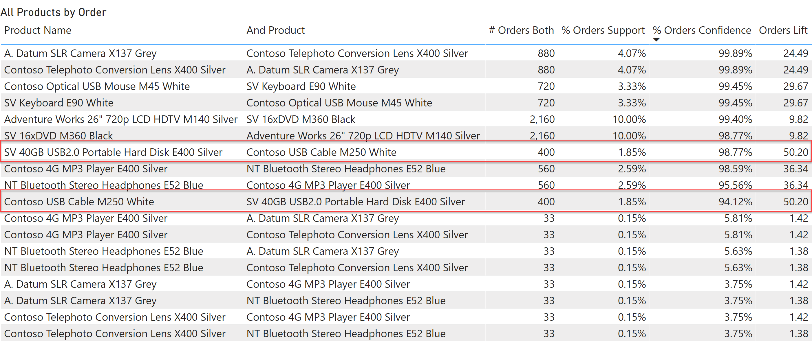
The dataset used in this example returns somewhat similar confidence values when the order of the two products is reversed. However, this is not common. Focus on the highlighted lines: when “Contoso USB Cable M250 White” is in the first column the confidence of an association with “SV 40GB USB2.0 Portable Hard Disk E400 Silver” is slightly smaller than the other way around. In real datasets, these differences are usually bigger. Even though support and lift are identical, the order matters for confidence.

The same pattern can use the customer as a basket instead of the order. By using the customer, there are many more products in each basket. With more data, it is possible to perform an analysis by category of product instead of by individual product. For example, the report in Figure 5 shows what the associations are between categories in the customers’ purchase history.

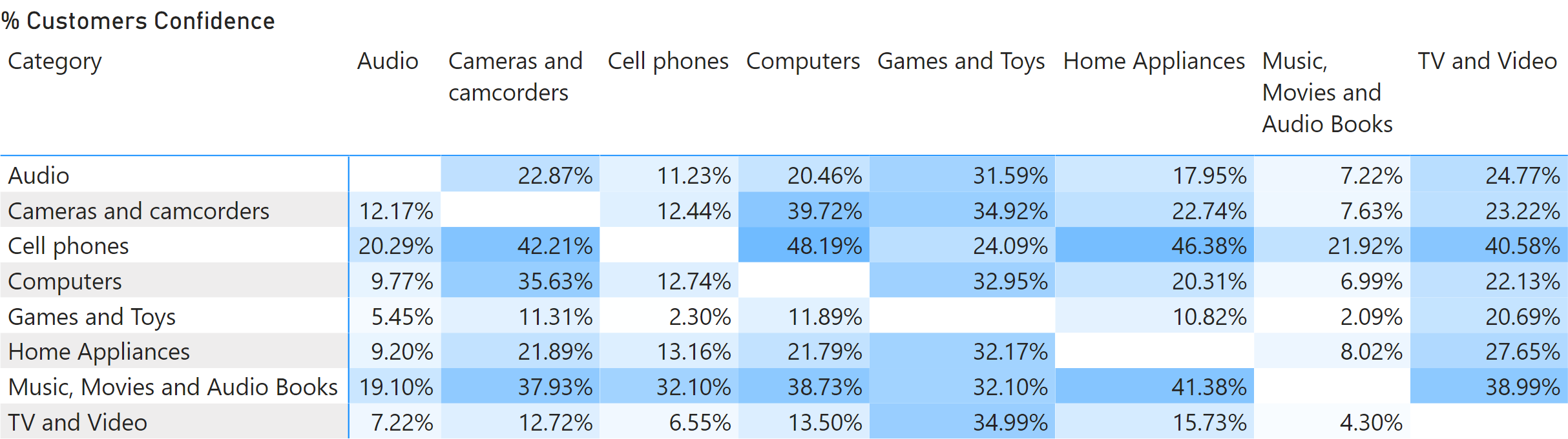
Customers buying “Cell phones” are likely to buy “Computers” too (confidence is 48.19%), whereas only 12.74% of customers buying “Computers” also buy “Cell phones”.

Basic pattern example

The model requires a copy of the Product table, needed to select the And Product in a report. The And Product table can be created as a calculated table using the following definition:

And Product = 
SELECTCOLUMNS (
    'Product',
    "And Category", 'Product'[Category],
    "And Subcategory", 'Product'[Subcategory],
    "And Product", 'Product'[Product Name],
    "And ProductKey", 'Product'[ProductKey]
)

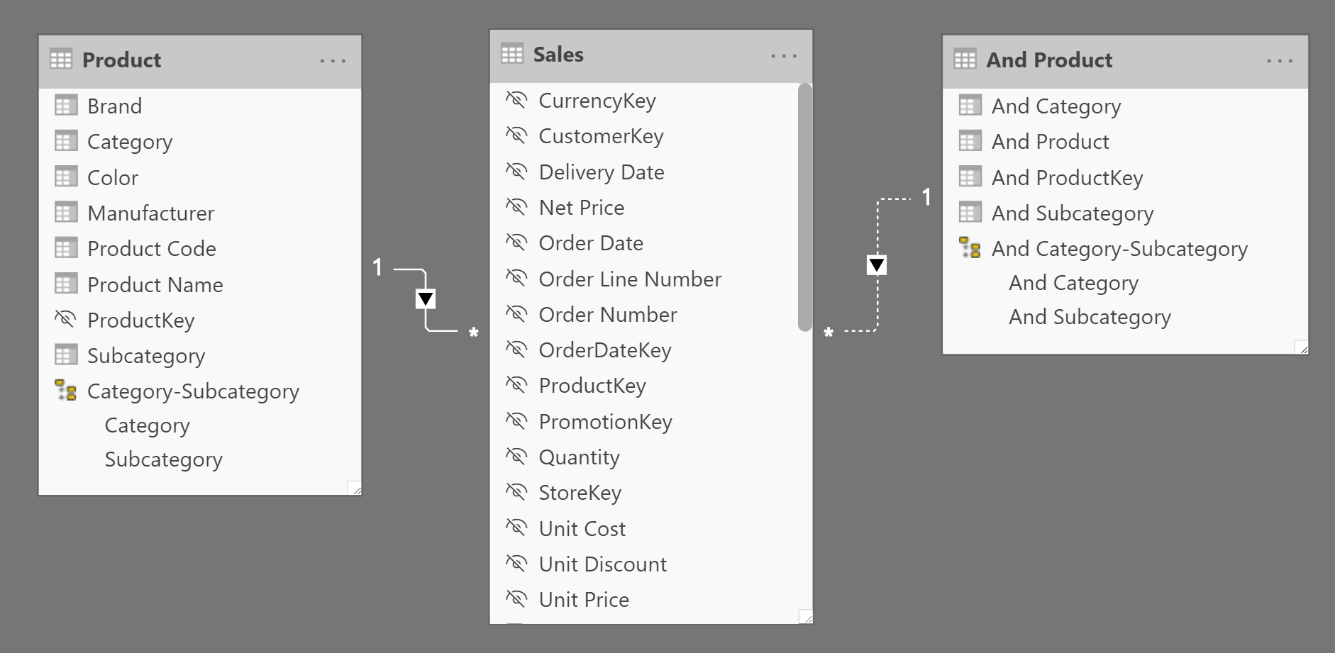
There is an inactive relationship between the And Product table and Sales, connecting the Sales[ProductKey] column used in the relationship between Product and Sales. The relationship must be inactive because it is only used in the measures of this pattern and should not affect other measures in the model. Figure 6 shows the relationships between Product, And Product, and Sales.

We use two baskets: orders and customers. An order is identified by Sales[Order Number], whereas a customer is identified by Sales[CustomerKey]. From now on, we show only the measures for orders, because the measures for the customers are a basic variation – obtained by replacing Sales[Order Number] with Sales[CustomerKey]. The curious reader can find the customer measures in the sample files.

The first measure counts the number of unique orders in the current filter context:

# Orders := 
SUMX ( SUMMARIZE ( Sales, Sales[Order Number] ), 1 )

Before we describe the remaining measures in the pattern, a small digression is required. The # Orders measure is actually a DISTINCTCOUNT over Sales[Order Number]. We used an alternative implementation for both flexibility and performance reasons. Let us elaborate on the rationale of this choice.

The # Orders measure could have been written using the following formula with DISTINCTCOUNT:

DISTINCTCOUNT ( Sales[Order Number] )

In DAX this is a shorter way to perform a COUNTROWS over DISTINCT:

COUNTROWS ( DISTINCT ( Sales[Order Number] ) )

You can replace DISTINCT with SUMMARIZE this way:

COUNTROWS ( SUMMARIZE ( Sales, Sales[Order Number] ) )

The last three versions of the formula return the same result in terms of performance and query plan. Using SUMX instead of COUNTROWS leads to the same result:

SUMX ( SUMMARIZE ( Sales, Customer[City] ), 1 )

Usually, replacing COUNTROWS with SUMX produces a query plan with lower performance. However, the specifics of Basket analysis make this alternative much faster in this pattern. More details about this optimization are available in this article: Analyzing the performance of DISTINCTCOUNT in DAX.

The advantage of using SUMMARIZE is that we can replace the second argument with a column that represents the basket even if it is in another table, as long as the table is related to Sales. For example, the measure computing the number of unique customer cities can be written this way:

SUMX ( SUMMARIZE ( Sales, Customer[City] ), 1 )

The first argument of SUMMARIZE needs to be the table containing the transactions, like Sales. If the second argument is a column in Customer, then you have no choice: you must use that column. For example, for the city of the customer you specify Customer[City]. In case you use the column that defines the relationship, like CustomerKey for Customer, then you can choose to use either Sales[CustomerKey] or Customer[CustomerKey]. Whenever possible, it is better to use the column available in Sales to avoid traversing the relationship. This is why instead of using Customer[CustomerKey] to identify the customer as a basket, we used Sales[CustomerKey]:

SUMX ( SUMMARIZE ( Sales, Sales[CustomerKey] ), 1 )

Now that we have explained why we use SUMMARIZE instead of DISTINCT to identify the basket attribute, we can move forward with the other measures of the pattern.

# Orders And computes the number of orders by using the selection made in And Product. It activates the inactive relationship between Sales and And Product:

# Orders And := 
CALCULATE (
    [# Orders],
    REMOVEFILTERS ( 'Product' ),
    USERELATIONSHIP ( Sales[ProductKey], 'And Product'[And ProductKey] )
)

# Orders Total returns the number of orders, while ignoring any selection in Product:

# Orders Total := 
CALCULATE (
    [# Orders], 
    REMOVEFILTERS ( 'Product' ) 
)

# Orders Both (Internal) is a hidden measure used to compute the number of orders including at least one item of Product and one item of And Product:

# Orders Both (Internal) := 
VAR OrdersWithAndProducts =
    CALCULATETABLE (
        SUMMARIZE ( Sales, Sales[Order Number] ),
        REMOVEFILTERS ( 'Product' ),
        REMOVEFILTERS ( Sales[ProductKey] ),
        USERELATIONSHIP ( Sales[ProductKey], 'And Product'[And ProductKey] )
    )
VAR Result =
    CALCULATE ( 
        [# Orders], 
        KEEPFILTERS ( OrdersWithAndProducts ) 
    )
RETURN
    Result

This hidden measure is useful to compute # Orders Both and other calculations described later in the optimized version of the pattern. # Orders Both adds a check to return blank in case the selection in Product and And Product contains at least one identical product. This is required to prevent the report from showing associations between a product and itself:

# Orders Both := 
IF (
    ISEMPTY (
        INTERSECT (
            DISTINCT ( 'Product'[ProductKey] ),
            DISTINCT ( 'And Product'[And ProductKey] )
        )
    ),
    [# Orders Both (Internal)]
)

% Orders Support is the ratio of # Orders Both to # Orders Total:

% Orders Support := 
DIVIDE ( [# Orders Both], [# Orders Total] )

% Orders Confidence is the ratio of # Orders Both to # Orders:

% Orders Confidence := 
DIVIDE ( [# Orders Both], [# Orders] )

Orders Lift is the result of the division of % Orders Confidence by the ratio of # Orders And to # Orders Total, as per the formula we had introduced earlier:

Orders Lift := 
DIVIDE (
    [% Orders Confidence],
    DIVIDE (
        [# Orders And],
        [# Orders Total]
    )
)

The code described in this section works. Yet, the measures might display performance issues in case there are more than a few thousand products. The optimized pattern provides a faster solution, but at the same time it requires additional calculated tables and relationships to improve the performance.

Optimized pattern example

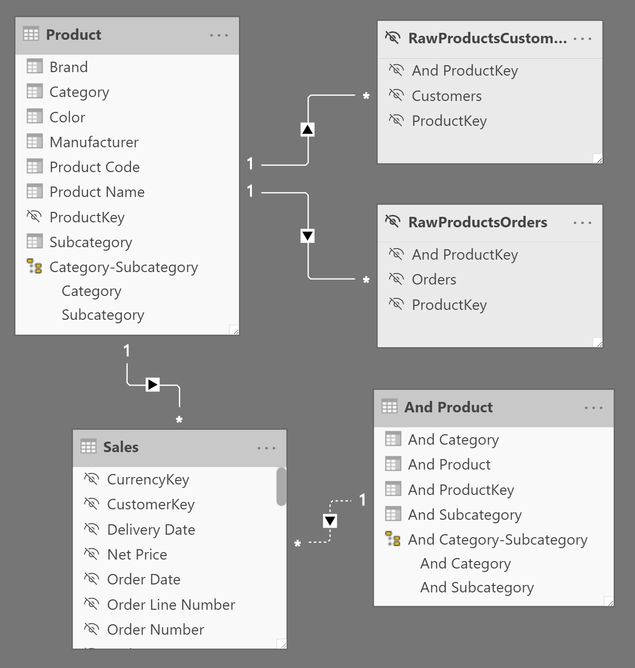
The optimized pattern reduces the effort required at query time to find the best combinations of products to consider. The performance improvement is obtained by creating calculated tables that pre-compute the existing combinations of products in the available baskets. Because we consider orders and customers as baskets, we created two calculated tables that are related to Product, as shown in Figure 7.

The RawProductsOrders and RawProductsCustomers tables contain in each row, a combination of two product keys alongside the number of baskets containing both products. The rows that would combine identical products are excluded:

RawProductsOrders = 
FILTER (
    SUMMARIZECOLUMNS (
        'Sales'[ProductKey],
        'And Product'[And ProductKey],
        "Orders", [# Orders Both (Internal)]
    ),
    NOT ISBLANK ( [Orders] ) && 'And Product'[And ProductKey] <> 'Sales'[ProductKey]
)

RawProductsCustomers = 
FILTER (
    SUMMARIZECOLUMNS (
        'Sales'[ProductKey],
        'And Product'[And ProductKey],
        "Customers", [# Customers Both (Internal)]
    ),
    NOT ISBLANK ( [Customers] ) && 'And Product'[And ProductKey] <> 'Sales'[ProductKey]
)

The filter from Product automatically propagates to the two RawProducts tables. Only the filter from And Product must be moved through a DAX expression in the # Orders Both measure. Indeed, # Orders Both is the only measure that differs from the ones in the basic pattern:

# Orders Both := 
VAR ExistingAndProductKey =
    CALCULATETABLE (
        DISTINCT ( RawProductsOrders[And ProductKey] ),
        TREATAS ( 
            DISTINCT ( 'And Product'[And ProductKey] ), 
            RawProductsOrders[And ProductKey] 
        )
    )
VAR FilterAndProducts =
    TREATAS (
        EXCEPT (
            ExistingAndProductKey,
            DISTINCT ( 'Product'[ProductKey] )
        ),
        Sales[ProductKey]
    )
VAR OrdersWithAndProducts =
    CALCULATETABLE (
        SUMMARIZE ( Sales, Sales[Order Number] ),
        REMOVEFILTERS ( 'Product' ),
        FilterAndProducts
    )
VAR Result =
    CALCULATE ( 
        [# Orders], 
        KEEPFILTERS ( OrdersWithAndProducts ) 
    )
RETURN
    Result

# Orders Both cannot use the # Orders Both (Internal) implementation because of the way it applies the filters. # Orders Both transfers the filter from And Product to RawProductsOrders and then to Sales in order to retrieve the orders that include any of the items in Any Product. This technique is somewhat complex, but it is useful in order to reduce the workload in the formula engine. All this results in better performance at query time.

DISTINCTCOUNT

Counts the number of distinct values in a column.

DISTINCTCOUNT ( <ColumnName> )

COUNTROWS

Counts the number of rows in a table.

COUNTROWS ( [<Table>] )

DISTINCT

Returns a one column table that contains the distinct (unique) values in a column, for a column argument. Or multiple columns with distinct (unique) combination of values, for a table expression argument.

DISTINCT ( <ColumnNameOrTableExpr> )

SUMMARIZE

Creates a summary of the input table grouped by the specified columns.

SUMMARIZE ( <Table> [, <GroupBy_ColumnName> [, [<Name>] [, [<Expression>] [, <GroupBy_ColumnName> [, [<Name>] [, [<Expression>] [, … ] ] ] ] ] ] ] )

SUMX

Returns the sum of an expression evaluated for each row in a table.

SUMX ( <Table>, <Expression> )