The Events in Progress pattern has a broad field of application. It is useful whenever dealing with events with a duration – events that have a start date and an end date. The event is considered to be in progress between the two dates. As an example, we use Contoso orders.

Each order has an order date and a delivery date. The date when the order was placed is considered the start date, and the date when the order was delivered is considered the end date. An order is considered open when it has been placed but has not yet been delivered. We are interested in counting how many orders are open at a certain date, and what their value is.

As with many of the patterns described, Events in Progress can be handled both dynamically through measures, or statically by using a snapshot table.

Definition of events in progress

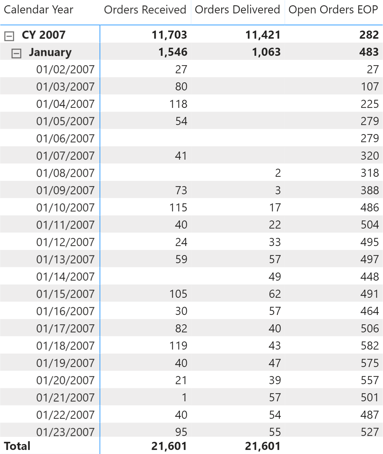
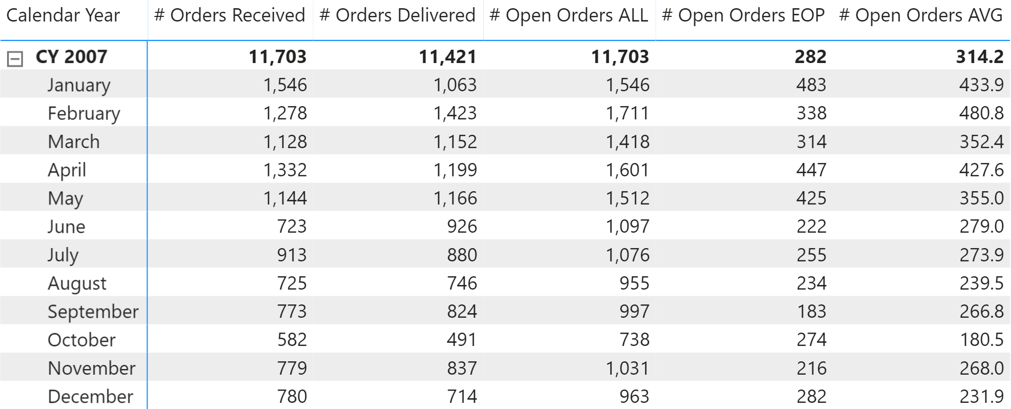
You need to compute how many orders are open at a specific time, for Contoso. In Figure 1 you can see the result of the calculation at the day level; on each day the number of open orders is the number open orders from the previous day, plus the orders received and minus the orders delivered that day. EOP stands for End Of Period.

However, this way of computing the number of open orders could be ambiguous when we consider a period of several days, such as a month or a year. The ambiguity is explained below. To avoid this ambiguity, it is important to clearly define the desired result. When looking at a single day, the number of orders open is evident, as you can see in Figure 2.

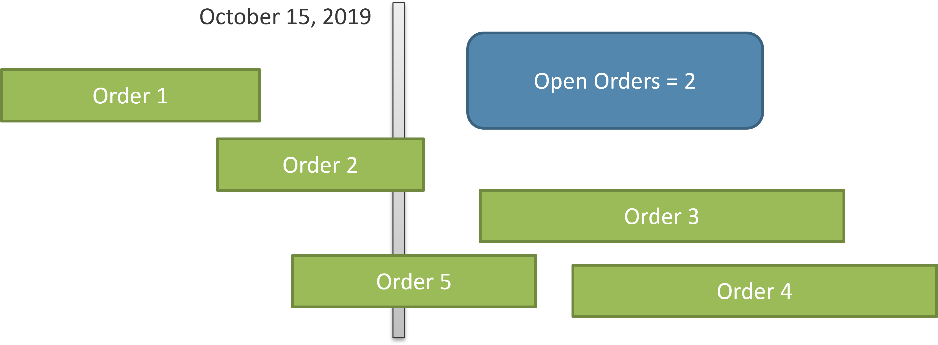
In Figure 2 only orders number 2 and 5 are open at the date considered (October 15, 2019). Order 1 is already delivered, whereas orders 3 and 4 are yet to be received by Contoso. Therefore, the calculation is clearly defined. Nevertheless, when you report on a larger period of time, like a month, the calculation is harder to define. Look at Figure 3 where the time duration is much larger, including the full month of October.

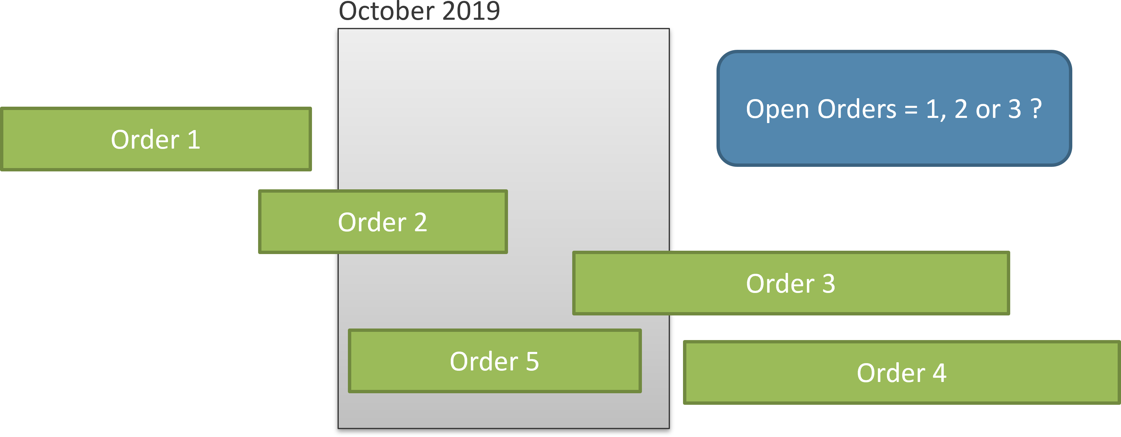
In Figure 3, order 1 is completed before the beginning of October, and order 4 is yet to be received by Contoso after the end of October. Therefore, their status is obvious. However, order 2 is open at the beginning of the month, but it is closed at the end. Order 3 is opened during the month and still open at the end of the month. Order 5 is received and closed during the month. As you see, a calculation that is straightforward on an individual day requires a better definition at an aggregate level.

We do not want to provide an extensive description of every possible option. In this pattern we only consider the following three definitions for the orders in a period longer than one day – each measure is identified with a suffix from the list:

• ALL: Returns the orders that were open at any time during the period. For Figure 3, we report three orders; we consider order 5 as open because it has been open for some time during the period considered.
• EOP: Considers the status of each order at the end of the period. For Figure 3, this means reporting only one order (order 3), because all the other orders are either closed or not yet opened at the end of the period.
• AVG: Computes the daily average of the orders open in the period. This requires computing the number of open orders day by day, and then averaging it over longer periods.

There might be different definitions of open orders, which usually are slight variations of the three scenarios described above.

Open orders

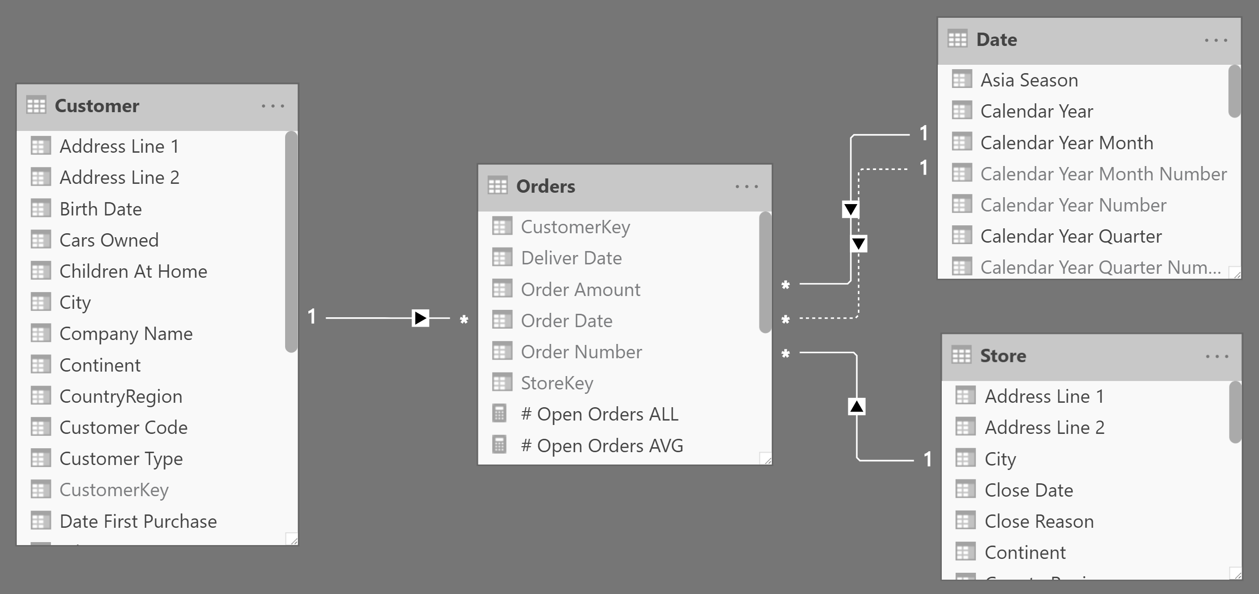
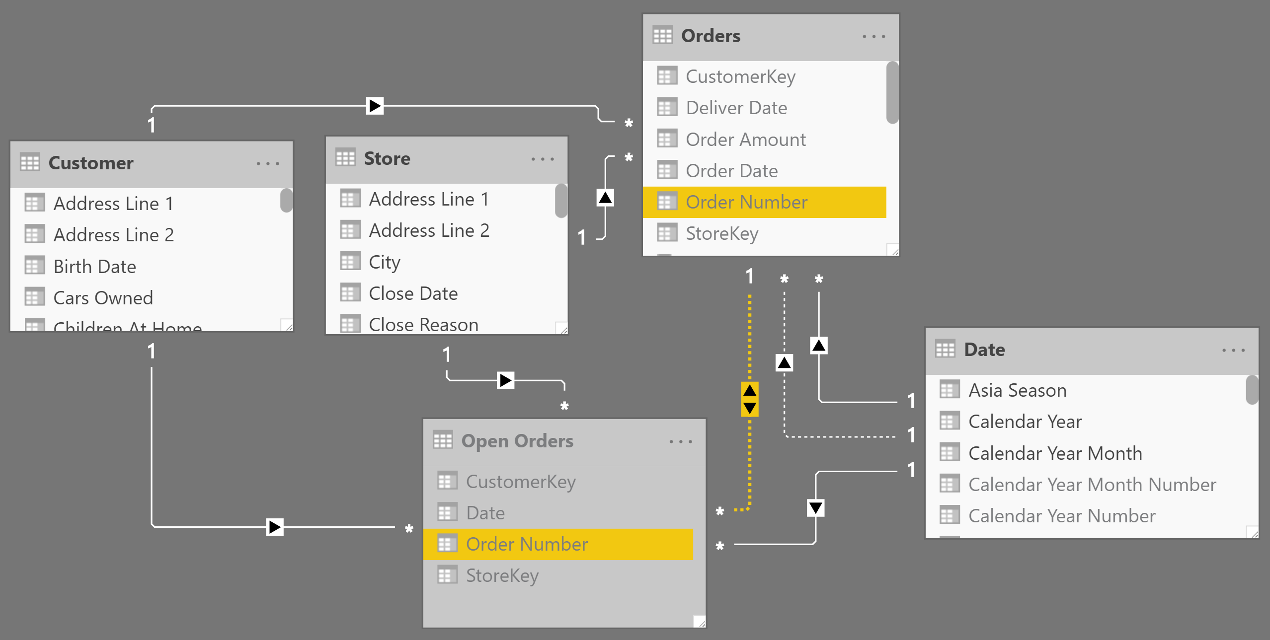
If the Orders table stores data at the correct granularity – storing one row for each order along with order date and delivery date – then the model looks like the one in Figure 4.

The DAX code computing the open orders for this model is rather simple:

# Open Orders ALL :=
VAR MinDate = MIN ( 'Date'[Date] )
VAR MaxDate = MAX ( 'Date'[Date] )
VAR Result =
    CALCULATE (
        COUNTROWS ( Orders ),
        Orders[Order Date] <= MaxDate,
        Orders[Deliver Date] > MinDate,
        REMOVEFILTERS ( 'Date' )
    )
RETURN
    Result

It is worth noting that REMOVEFILTERS is required, in order to remove any report filters that may be affecting the Date table.

Based on this measure, you can compute the two variations (end of period and average) using the following formulas:

# Open Orders EOP := 
CALCULATE (
    [# Open Orders ALL],
    LASTDATE ( 'Date'[Date] ) 
)

# Open Orders AVG := 
AVERAGEX ( 
    'Date', 
    [# Open Orders ALL] 
)

You can see the result of these formulas in Figure 5.

The Orders table might have more than one row for each order. If the Orders table has one row for each line in the order instead of one row for each order, then you should use DISTINCTCOUNT over a column containing a unique identifier for each order – instead of using COUNTROWS over the Orders table. This is not the case in our sample model, but in that scenario the # Open Orders ALL formula would differ by just one line:

# Open Orders ALL :=
VAR MinDate = MIN ( 'Date'[Date] )
VAR MaxDate = MAX ( 'Date'[Date] )
VAR Result =
    CALCULATE (                                 -- If any order can have several rows
        DISTINCTCOUNT ( Orders[Order Number] ), -- use DISTINCTCOUNT instead of COUNTROWS 
        Orders[Order Date] <= MaxDate,
        Orders[Deliver Date] > MinDate,
        REMOVEFILTERS ( 'Date' )
    )
RETURN
    Result

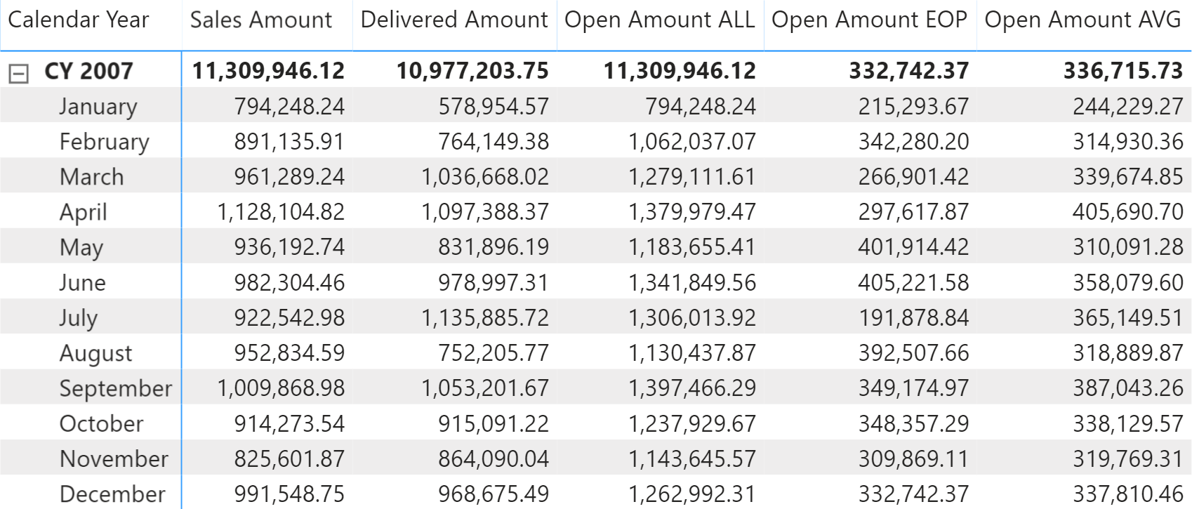
If you want to compute the dollar value of the open orders, you use the Sales Amount measure instead of the COUNTROWS or DISTINCTCOUNT functions. For example, this is the definition of the Open Amount ALL measure:

Open Amount ALL :=
VAR MinDate = MIN ( 'Date'[Date] )
VAR MaxDate = MAX ( 'Date'[Date] )
VAR Result =
    CALCULATE (
        [Sales Amount],        -- Use Sales Amount instead of DISTINCTCOUNT or COUNTROWS 
        Orders[Order Date] <= MaxDate,
        Orders[Deliver Date] > MinDate,
        REMOVEFILTERS ( 'Date' )
    )
RETURN
    Result

The other two measures just reference the underlying Open Amount ALL measure instead of # Open Orders ALL:

Open Amount EOP := 
CALCULATE (
    [Open Amount ALL],
    LASTDATE ( 'Date'[Date] ) 
)

Open Amount AVG := 
AVERAGEX ( 
    'Date', 
    [Open Amount ALL] 
)

The Figure 6 shows the results of the measures defined above.

The formulas described in this section work well on small datasets, but they require a big effort from the Formula Engine; this results in reduced performance starting from medium-sized databases and above – think hundreds of thousands of orders. If you need better performance, using a snapshot table is a very good option.

Open orders with snapshot

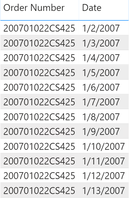
Building a snapshot simplifies the calculation and speeds up the performance. A daily snapshot contains one row per day and order that is open on that day. Therefore, a single order that has been open for 10 days requires 10 rows in the snapshot.

In Figure 7 you can see an excerpt from the snapshot table.

For large data models where the snapshot requires tens of millions of rows, it is suggested to use specific ETLs or queries in SQL to get the snapshot result. For smaller data models, the snapshot table can be created by using either Power Query or DAX. For example, the snapshot of our sample model can be created using the following definition of the Open Orders calculated table:

Open Orders =
SELECTCOLUMNS (
    GENERATE (
        Orders,
        DATESBETWEEN (
            'Date'[Date],
            Orders[Order Date],
            Orders[Deliver Date] - 1
        )
    ),
    "StoreKey", Orders[StoreKey],
    "CustomerKey", Orders[CustomerKey],
    "Order Number", Orders[Order Number],
    "Date", 'Date'[Date]
)

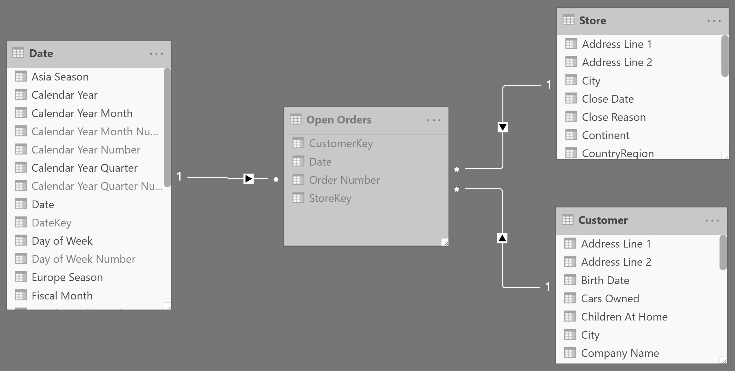
In Figure 8 you can see that the Open Orders snapshot has a set of regular relationships with the other tables in the model.

Using the snapshot, the formulas that compute the number of open orders are faster and simpler to write:

# Open Orders ALL := 
DISTINCTCOUNT ( 'Open Orders'[Order Number] )

# Rows Open Orders := 
COUNTROWS ( 'Open Orders' )

# Open Orders EOP := 
CALCULATE ( 
    [# Rows Open Orders], 
    LASTDATE ( 'Date'[Date] ) 
)

# Open Orders AVG := 
AVERAGEX ( 
    'Date', 
    [# Rows Open Orders] 
)

Only the # Open Orders ALL measure requires the DISTINCTCOUNT function. The other two measures, # Open Orders EOP and # Open Orders AVG count the number of open orders one day at a time, which can be done using a faster COUNTROWS over the snapshot table.

The Open Amount ALL measure requires you to apply the list of open orders as a filter to the Orders table. This is achieved using TREATAS:

Open Amount ALL := 
VAR OpenOrders =
    DISTINCT ( 'Open Orders'[Order Number] )
VAR FilterOpenOrders = 
    TREATAS (
        OpenOrders,
        Orders[Order Number]
    )
VAR Result =
    CALCULATE (
        [Sales Amount],
        FilterOpenOrders,
        REMOVEFILTERS ( Orders )
    )
RETURN Result

The Open Amount EOP and Open Amount AVG measures just reference the underlying Open Amount ALL measure instead of # Open Orders ALL:

Open Amount EOP := 
CALCULATE ( 
    [Open Amount ALL], 
    LASTDATE ( 'Date'[Date] ) 
)

Open Amount AVG := 
AVERAGEX ( 
    'Date', 
    [Open Amount ALL] 
)

The size of the snapshot depends on the number of orders and on the average duration of an order. If an order typically stays open for a few days, then it is fine to use a daily granularity. If an order is usually active for a much longer period of time (think years) then you should consider moving the snapshot granularity to the month level – one row for each order open in each month.

A possible optimization requires an inactive relationship between Orders and Open Orders. This is only useful when the Orders table has one row per order – the Orders[Order Number] column is thus unique and the relationship has a one-to-many cardinality. The inactive relationship should be like the one highlighted in Figure 9. Do not use this technique with a many-to-many cardinality because the pure DAX approach based on TREATAS would be similar in performance and simpler to manage.

Then you should replace the previous Open Amount ALL measure with the code of the Open Amount ALL optimized measure defined as follows:

Open Amount ALL optimized :=
CALCULATE (
    [Sales Amount],
    USERELATIONSHIP ( 'Open Orders'[Order Number], Orders[Order Number] ),
    CROSSFILTER ( Orders[Order Date], 'Date'[Date], NONE )
)

Leveraging the relationship to transfer the filter reduces the workload of the Formula Engine and improves the performance of all the measures based on Open Amount ALL. You should just consider the side effects of USERELATIONSHIP in different models, applying the required CROSSFILTER to remove possible ambiguities. Usually it should be enough to disable the relationship between Orders and Date like in this example, but carefully check the accuracy of the results by comparing the optimized measure with the one based on TREATAS.

ALL

CALCULATE modifier

Returns all the rows in a table, or all the values in a column, ignoring any filters that might have been applied.

ALL ( [<TableNameOrColumnName>] [, <ColumnName> [, <ColumnName> [, … ] ] ] )

REMOVEFILTERS

CALCULATE modifier

Clear filters from the specified tables or columns.

REMOVEFILTERS ( [<TableNameOrColumnName>] [, <ColumnName> [, <ColumnName> [, … ] ] ] )

DISTINCTCOUNT

Counts the number of distinct values in a column.

DISTINCTCOUNT ( <ColumnName> )

COUNTROWS

Counts the number of rows in a table.

COUNTROWS ( [<Table>] )

TREATAS

Treats the columns of the input table as columns from other tables.For each column, filters out any values that are not present in its respective output column.

TREATAS ( <Expression>, <ColumnName> [, <ColumnName> [, … ] ] )

USERELATIONSHIP

CALCULATE modifier

Specifies an existing relationship to be used in the evaluation of a DAX expression. The relationship is defined by naming, as arguments, the two columns that serve as endpoints.

USERELATIONSHIP ( <ColumnName1>, <ColumnName2> )

CROSSFILTER

CALCULATE modifier

Specifies cross filtering direction to be used in the evaluation of a DAX expression. The relationship is defined by naming, as arguments, the two columns that serve as endpoints.

CROSSFILTER ( <LeftColumnName>, <RightColumnName>, <CrossFilterType> )