Budget

This pattern includes several coding techniques you may find useful for budgeting scenarios. The techniques do not apply only to budgeting. We use the budget as an example to show how to reallocate a measure at a different granularity, and how to combine measures coming from tables with different granularities into the same chart.
Besides, each company has its own approach for creating and managing a budget. This pattern is just an example of what can be done. You must adapt the measures and the techniques shown in this pattern to your specific business.
Introduction
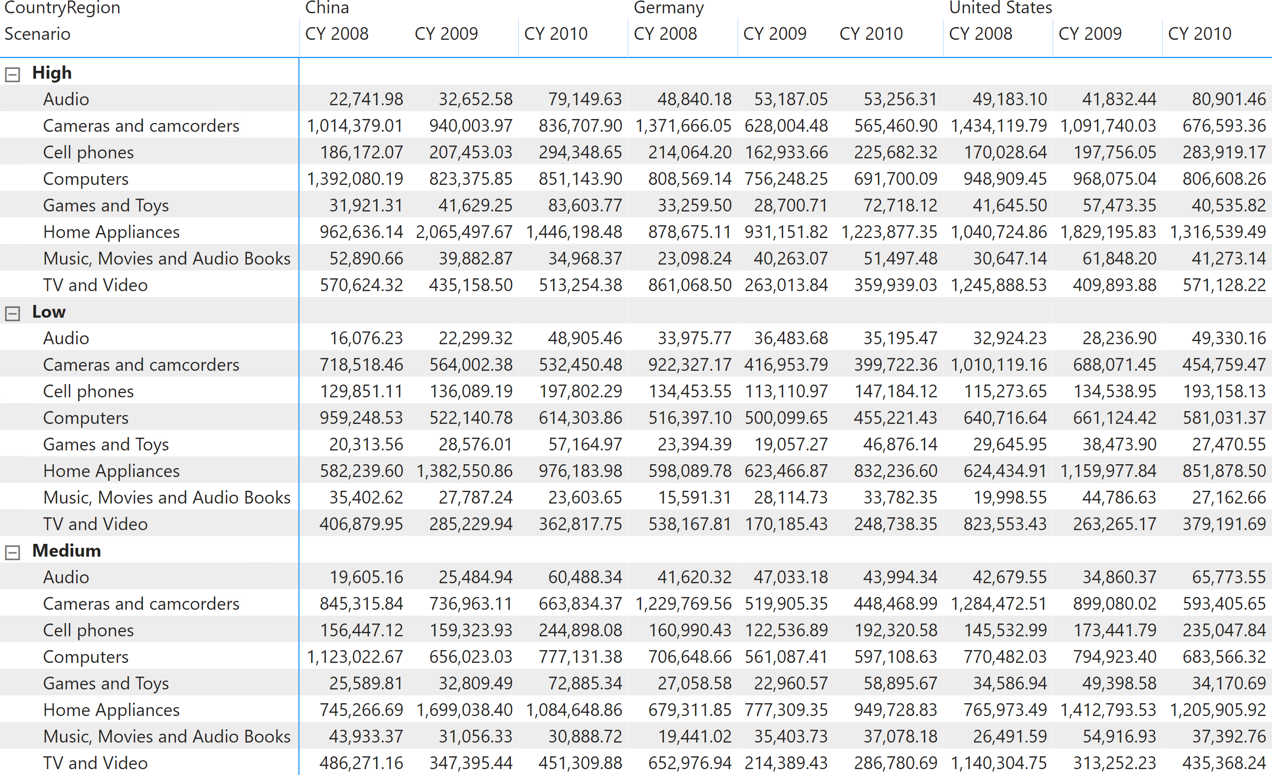
The initial table used for the budget contains forecasts of sales at a certain granularity. In our example, this table contains forecasts of sales by store country, product category, and year. There are three forecasts named Low, Medium, and High. Figure 1 shows the full dataset.
Based on this dataset, we work with the following requirements:
- Allocating the forecast at a different granularity. For example, computing the monthly forecast based on the sales in the previous year.
- Combining actuals and forecasts in the same report, using the actual values for the past months and the forecasts for the future months of the current year.
- Correcting the forecast of future months based on how far they are from the actuals in past months of the current year.
Additionally, we want to keep in mind new products that might be introduced throughout the years, as well as discontinued products for which the forecast should not be computed. For this purpose, we use a table called Override that states when a product was introduced, along with the sales forecast for the first year. The same Override table also includes the dismission date of the discontinued products that are not used in order to allocate the forecast. The allocation of the new products by store country must be based on past sales of other products.
The data model
Before diving into the details of the calculations, it is important to make some considerations about the data model.
The scenario we are analyzing is a top-down forecasting scenario. Therefore, the source data contains a forecast of sales for different scenarios at a low granularity. Low granularity means that the information provided is at a very high level: year, store country, and product category. There are no details about individual products, months or stores. Consequently, the Forecast table is linked with the relevant tables using weak Many-Many-Relationships (MMR) and it has a Single-Many-Relationship (SMR) only with the Scenario table, as depicted in the diagram in Figure 2.
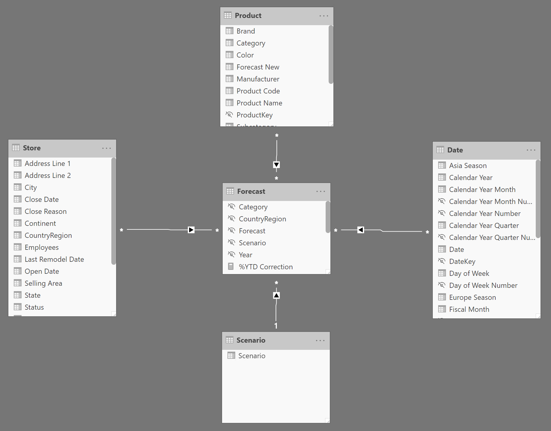
The following relationships start off of the Forecast table:
- MMR with Store based on the CountryRegion
- MMR with Product based on the Category
- MMR with Date based on the Year
- SMR with Scenario based on the Scenario
All the MMRs are weak relationships; they only filter at the granularity of the relationship. At a more detailed (higher) granularity, they just repeat the total at the supported grain.
NOTE The use of MMR and SMR is required to avoid confusion with other definitions of many-to-many relationships. A complete description of the MMR and SMR relationships in Power BI is available in the Relationships in Power BI and Tabular models article.
The Scenario table implements the best practice of always using dimension tables to slice and dice, instead of using columns in the fact table (Forecast in this case) for slicers and filters.
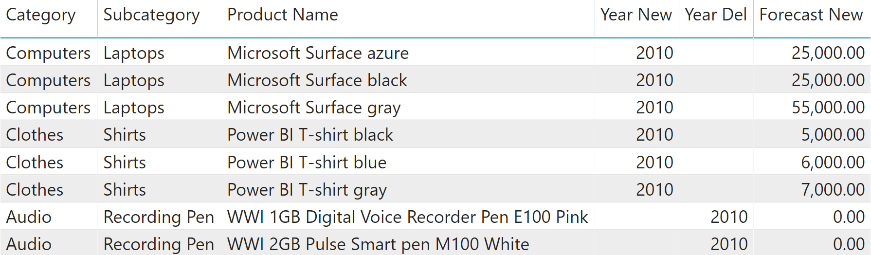
The forecast information of this pattern comes from an Excel file. The same Excel file includes another table called Override, which contains information about new and dismissed products. The relevant columns in the Override table are:
- Year New: the year a new product was introduced.
- Year Del: the year a product was (or will be) dismissed.
- Amount: the forecast sales over all countries for the first year.
Because the Override table has the same granularity as the Product table, we used Power Query to merge these three columns directly in the Product table. Figure 3 shows the content of these three columns imported in Product from the Override table.
This is not necessarily an optimal model. We designed it to show you the DAX code, but different requirements might justify using a different model. You should update the calculations to reflect your specific requirements and data model.
Business choices
As with the model, we needed to set some business choices in order to author the DAX code. The following sections describe the business rules implemented in this pattern.
Allocation based on the previous year
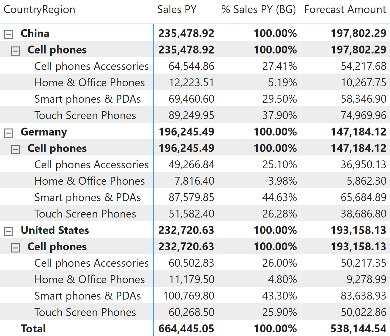
When the forecast needs to be reallocated, we consider the sales in the previous year as an allocation factor. In other words, in order to show the forecast of a subcategory, we reallocate the budget defined at the category level by the percentage of sales of the given subcategory against the corresponding category in the previous year.
This is better depicted in Figure 4.
Consequently, a previously existing product that had no sales in one year, will have a forecast of zero in the following year.
Dismissed products do not contribute to the allocation
If a product is dismissed, its forecast for the new year is zero since the product is no longer available for sale. Consequently, the forecast for the new year does not include dismissed products. If we ignored this condition, the allocation would produce undesired results.
For example, think about what would happen if all the products in the category Cell Phones Accessories were dismissed. In the United States, they contribute for 26% of sales, as shown in Figure 4. Because the products of this category are dismissed, the forecast for the next year does not include their sales. The allocation formula must take this into account, by increasing the percentages of other subcategories to compensate for the absence of a certain category. If not, the total allocated forecast would only add up to 74% of the total forecast, hiding the 26% that are no longer being allocated to dismissed products.
In summary, if a product is dismissed one year, its sales in the previous year are not considered for the forecast allocation.
New products have their own forecast amount
This is not really a business decision, but rather a choice to simplify the model. If a product is being introduced as new, then its sales in the previous year are at zero. As we stated earlier, this would translate into an empty forecast for the following year. Still, the product being new is expected to have no sales in the previous year.
For this reason, every new product has a forecast amount associated to it for the year when it is being introduced. This is a single value, which is allocated in different store countries depending on the distribution percentage of all the other products over the store countries.
As with other options, this is not necessarily the best choice; but we must make a choice in order to write working code. In other scenarios, there could be a table containing more detailed forecasts, or the issue could be ignored for a specific business. Therefore, consider this as an optional implementation option and not as a mandatory requirement.
Products can be dismissed or introduced on a yearly basis
In order to keep the model simple enough, we introduced this artificial limitation: a product is introduced at the beginning of a year (therefore it starts selling in January) and dismissed at the end of a year (no more sales in the new year).
Handling the introduction of products at different points in time introduces a new level of complexity around time. Indeed, when computing the forecast for the new products, the amount should be allocated only starting at a given point in time. Dismissed products present a similar issue. We decided not to handle this complexity in order to focus more on the allocation algorithm. Specific and more detailed business requirements might require some adjustment to the proposed formulas.
Forecast allocation
The allocation of forecast uses sales in the previous year to determine the percentage of the total forecast that must be allocated to the current selection. The formula is composed of two main sections: the allocation of the forecast and the computation of the value for new products.
Figure 5 helps us better understand the calculation by showing the Forecast Amount and the % Sales PY (BG) measures side by side. % Sales PY (BG) is the allocation percentage at the budget granularity that is internally computed in Forecast Amount. The sample file includes a separate definition of % Sales PY (BG) just to display this intermediate calculation that is not relevant to the pattern.
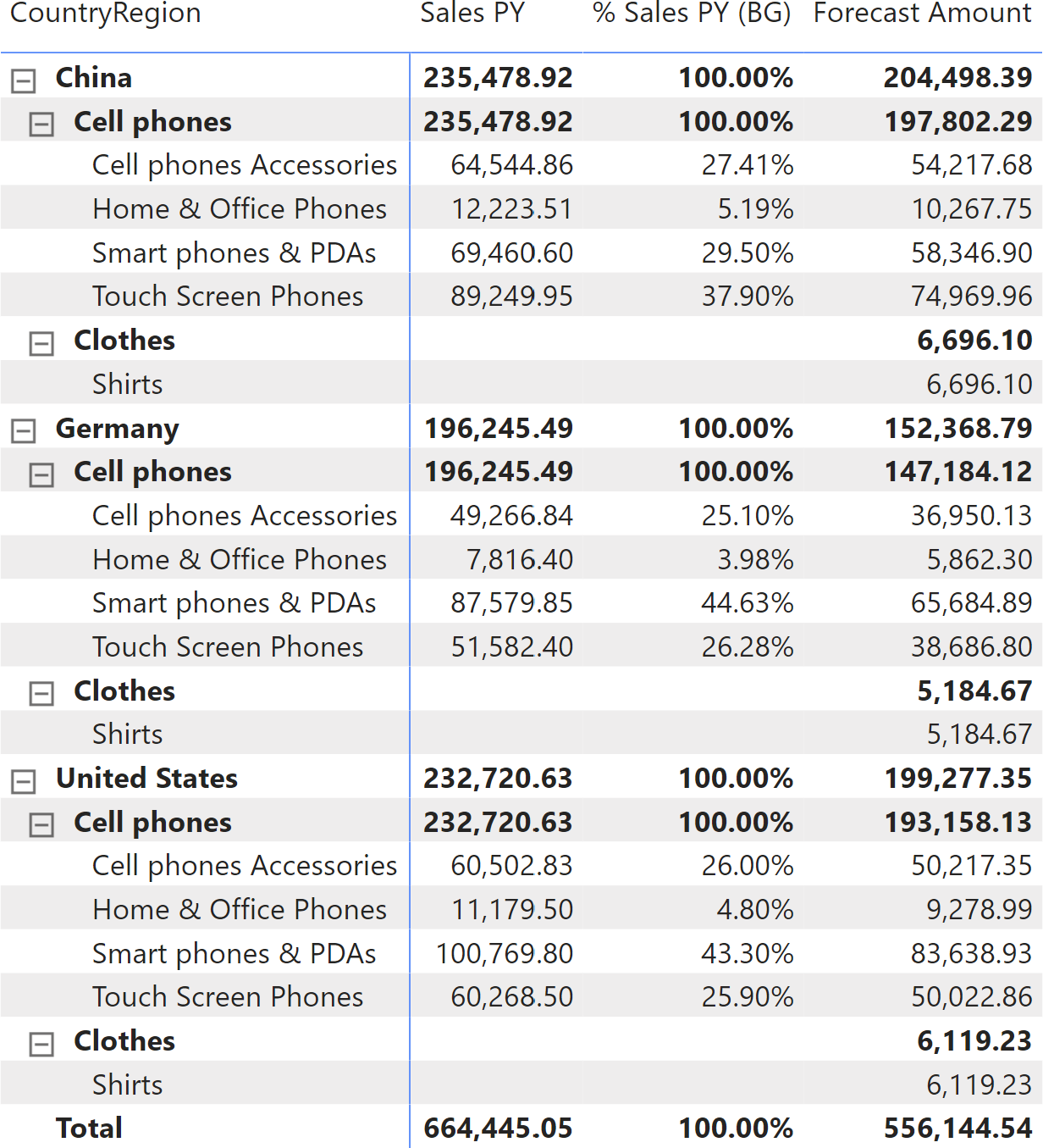
There are two categories selected in the report: Cell phones and Clothes. Clothes is a new category, that was not present in the previous year. The full forecast for each store country (China and Germany are visible in Figure 5) includes the allocated forecast for the selected country, plus the amount assigned to new products through the Forecast New column imported from the Amount column in the Override table of the Excel file.
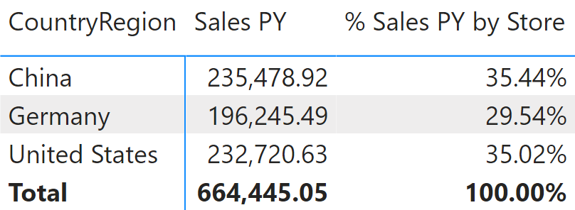
The model is designed in a way that there is a single forecast amount for each product for the entire year. This number must be allocated by store country based on the sales of the previous year for that country, as shown by % Sales PY by Store in Figure 6. This time, the allocation is made only by store country – no other columns are involved.
This is the definition of the Forecast Amount measure:
Forecast Amount :=
IF (
    HASONEVALUE( 'Date'[Calendar Year Number] ),
    VAR SelectedScenario = SELECTEDVALUE ( Scenario[Scenario], "Medium" )
    VAR Categories = VALUES ( 'Product'[Category] )
    VAR Countries = VALUES ( Store[CountryRegion] )
    VAR CurrentYear = VALUES ( 'Date'[Calendar Year Number] )

    --  Here we compute the PY sales amount at the forecast granularity,
    --  that is Category, CountryRegion, and Year. We do this by removing
    --  any filter on the granularity tables and then by restoring only
    --  the filters corresponding to the forecast granularity.
    VAR PYSalesAmountAtGrain =
        CALCULATE (
            [Sales PY],
            REMOVEFILTERS ( 'Product' ),
            REMOVEFILTERS ( 'Store' ),
            REMOVEFILTERS ( 'Date' ),
            Categories,
            Countries,
            CurrentYear,
            KEEPFILTERS ( 'Product'[Year Del] >= CurrentYear || ISBLANK ( 'Product'[Year Del] ) )
        )

    --  No special treatment for the forecast amount, as it is already at the
    --  Category, CountryRegion, and Year granularity despite any further filter.
    VAR CurrentForecastedAmount =
        CALCULATE (
            SUM ( Forecast[Forecast] ),
            Scenario[Scenario] = SelectedScenario
        )
    VAR CategoriesCountries =
        CROSSJOIN ( Categories, Countries )

    --  To compute the forecast value we iterate over categories and countries (note
    --  that there is always a single year selected, no need to iterate on that),
    --  we compute the sales amount at the Category/Country level. Then, we divide
    --  the result by the sales amount at the forecast granularity to obtain the
    --  percentage to allocate the forecast.
    --  The filter on Product[Year Del] guarantees that products removed before
    --  the current year are not being considered, as they will have no forecast amount.
    VAR ForecastValue =
        CALCULATE (
            SUMX (
                KEEPFILTERS ( CategoriesCountries ),
                VAR PYSalesAmount =  [Sales PY]
                VAR AllocationFactor = DIVIDE ( PYSalesAmount,  PYSalesAmountAtGrain )
                RETURN AllocationFactor * CurrentForecastedAmount
            ),
            KEEPFILTERS ( 'Product'[Year Del] >= CurrentYear || ISBLANK ( 'Product'[Year Del] ) )
        )
    --  Now we determine the amount of new products, which must be allocated
    --  by country using the sales of any product in the same period in the
    --  previous year.
    VAR NewProductsAmount =
        CALCULATE (
            SUM ( 'Product'[Forecast New] ),
            KEEPFILTERS ( 'Product'[Year Del] >= CurrentYear || ISBLANK ( 'Product'[Year Del] ) )
        )

    --  Here we compute the PY sales at the forecast granularity, regardless of
    --  any product and country, because the forecast for a new product is specified
    --  as a single number that sums sales in all the countries.
    VAR PYSalesAmountAtGrainAnyProduct =
        CALCULATE (
            [Sales PY],
            REMOVEFILTERS ( 'Product' ),
            REMOVEFILTERS ( 'Store' ),
            REMOVEFILTERS ( 'Date' ),
            CurrentYear
        )

    --  Similarly to what we did with the forecast, we allocate the new value.
    --  This time we need to iterate only on Countries, as there is only one year
    --  and categories should not be part of the iteration
    VAR NewValue =
        SUMX (
            KEEPFILTERS ( Countries ),
            VAR PYSalesAmountAnyProduct =
                CALCULATE (
                    [Sales PY],
                    REMOVEFILTERS ( 'Product' )
                )
            VAR AllocationFactor =
                DIVIDE ( PYSalesAmountAnyProduct,  PYSalesAmountAtGrainAnyProduct  )
            RETURN
                AllocationFactor * NewProductsAmount
        )
    --
    --  The result is the forecast value plus the value of new products, both reallocated
    --  according to different business requirements.
    --
    VAR Result =
        ForecastValue + NewValue
    RETURN
        Result
)
The formula works with a single year selected and it also produces correct results with a reduced set of dates within one year. It is also possible to implement time intelligence calculations over the Forecast Amount measures, like the year-to-date in the YTD Forecast measure:
YTD Forecast :=
CALCULATE (
    [Forecast Amount],
    DATESYTD ( 'Date'[Date] )
)
Showing actuals and forecasts on the same chart
A common requirement is to show both actual and forecast measures in the same chart. This type of requests might end up in producing reports that are not very useful, like the one visible in Figure 7. The YTD Sales (not filtered) measure displays the year-to-date of Sales Amount: because the Sales table contains data until August 14, 2010, the year-to-date is a flat line from August to December.
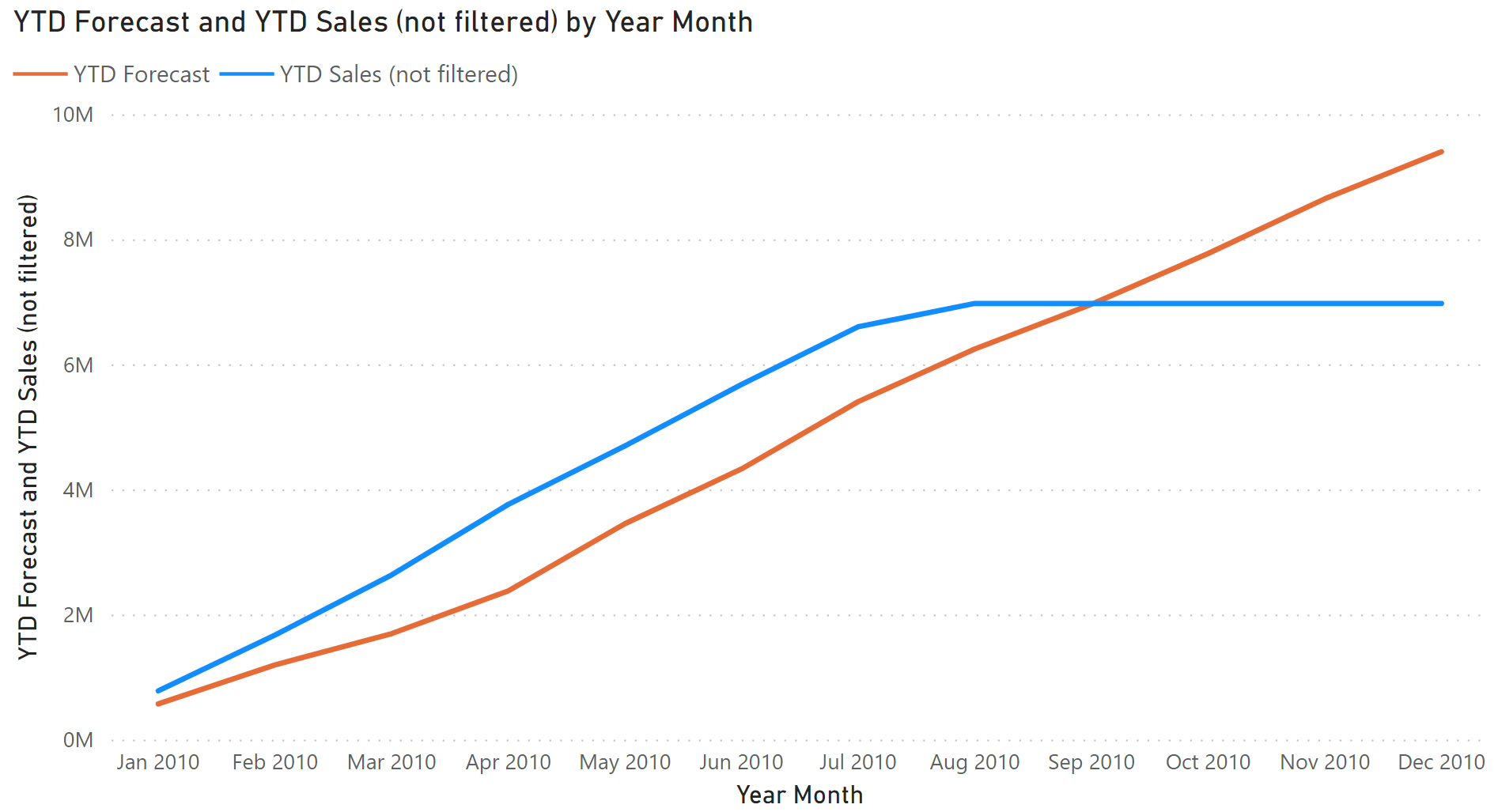
A better visualization in these cases shows the actual sales amount up to the last day of sales available, and then it uses the forecast for the following days to complete the chart for the future months. Figure 8 shows this type of report through a line chart.
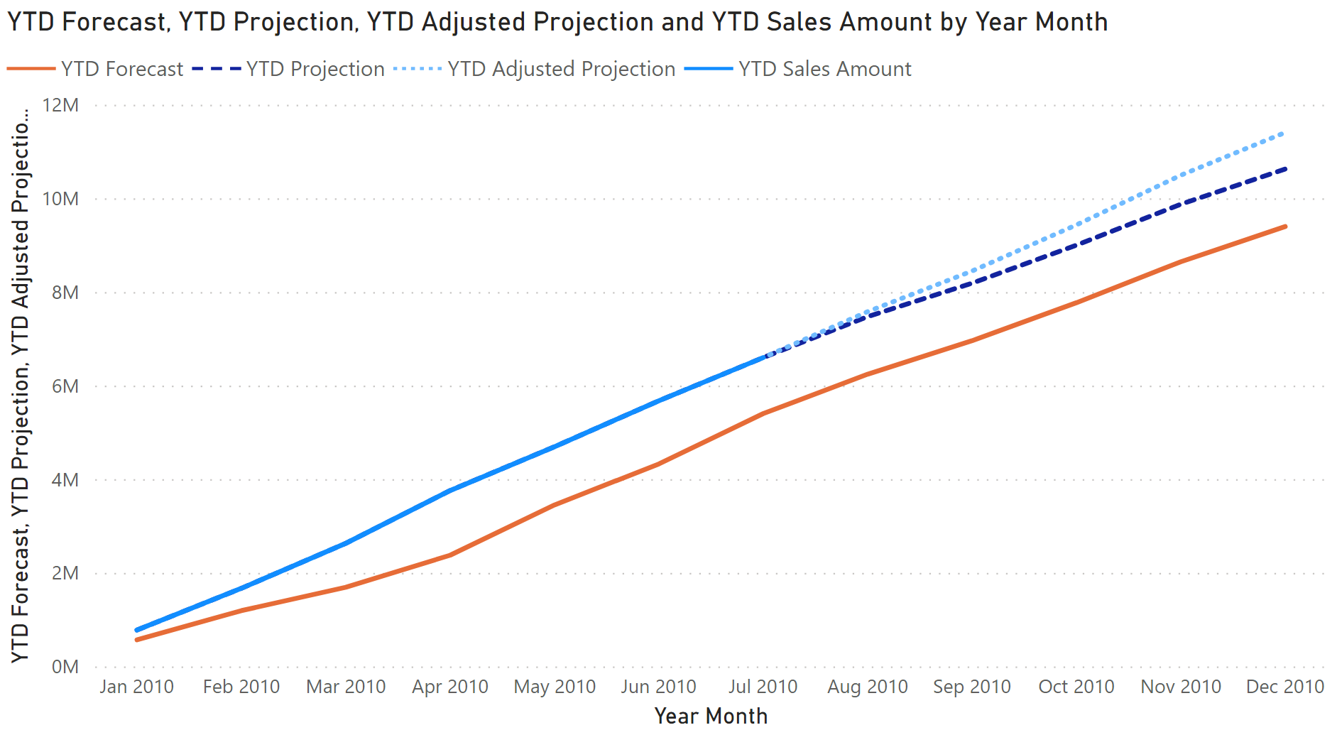
The last complete month showing data for the YTD Sales Amount measure is July 2010. The following months are not displayed thanks to the date check in the following implementation:
YTD Sales Amount :=
VAR LastAvailableDate =
    CALCULATE (
        MAX ( Sales[Order Date] ),
        REMOVEFILTERS ( 'Date' )
    )
VAR LastVisibleDate =
    MAX ( 'Date'[Date] )
VAR Result =
    IF (
        LastVisibleDate <= LastAvailableDate,
        CALCULATE ( [Sales Amount], DATESYTD ( 'Date'[Date] ) )
    )
RETURN
    Result
The YTD Forecast measure is only used to display the complete forecast in the line chart; It just computes the year-to-date of Forecast Amount defined in the previous section:
YTD Forecast :=
CALCULATE (
    [Forecast Amount],
    DATESYTD ( 'Date'[Date] )
)
The YTD Projection measure computes the year-to-date of the Projection Amount measure. The latter uses Sales Amount for the dates available in the Sales table (until August 14, 2010 in this example) and Forecast Amount for the dates following the last date available in Sales (dates greater than August 14, 2010 in this example):
YTD Projection :=
CALCULATE (
    [Projection Amount],
    DATESYTD ( 'Date'[Date] )
)
Projection Amount :=
VAR LastAvailableDate =
    CALCULATE (
        MAX ( Sales[Order Date] ),
        REMOVEFILTERS ( 'Date' )
    )
VAR ActualSalesAmount = [Sales Amount]
VAR ForecastedAmount =
    CALCULATE (
        [Forecast Amount],
        KEEPFILTERS ( 'Date'[Date] > LastAvailableDate )
    )
VAR Result =
    ActualSalesAmount + ForecastedAmount
RETURN
    Result
The YTD Adjusted Projection measure is like YTD Projection; however, it applies an adjustment factor to the Forecast Amount based on the comparison between available transactions and the corresponding forecast:
YTD Adjusted Projection :=
CALCULATE (
    [Adjusted Projection Amount],
    DATESYTD ( 'Date'[Date] )
)
Adjusted Projection Amount :=
VAR LastAvailableDate =
    CALCULATE (
        MAX ( Sales[Order Date] ),
        REMOVEFILTERS ( 'Date' )
    )
VAR ActualSalesAmount = [Sales Amount]
VAR AdjustmentFactor = [% Adjustment]
VAR ForecastAmount =
    CALCULATE (
        [Forecast Amount] * AdjustmentFactor,
        KEEPFILTERS ( 'Date'[Date] > LastAvailableDate )
    )
VAR Result =
    ActualSalesAmount + ForecastAmount
RETURN
    Result
The adjustment factor computed by the % Adjustment measure could have many different implementations, depending on specific business requirements. In this example we use the ratio between Sales Amount and Forecast Amount for the dates available in the Sales table:
% Adjustment :=
VAR LastAvailableDate =
    CALCULATE (
        MAX ( Sales[Order Date] ),
        REMOVEFILTERS ( 'Date' )
    )
VAR CurrentYear =
    SELECTEDVALUE ( 'Date'[Calendar Year] )
VAR Result =
    CALCULATE (
        DIVIDE (
            [Sales Amount],
            [Forecast Amount]
        ),
        'Date'[Date] <= LastAvailableDate,
        'Date'[Calendar Year] = CurrentYear
    )
RETURN
    Result
This pattern is designed for Power BI / Excel 2016-2019. An alternative version for Excel 2010-2013 is also available.
This pattern is included in the book DAX Patterns, Second Edition.


Video

Do you prefer a video?
This pattern is also available in video format. Take a peek at the preview, then unlock access to the full-length video on SQLBI.com.Watch the full video — 45 min.
Downloads
Download the sample files for Power BI / Excel 2016-2019: