Week-related calculations

This pattern describes how to compute week-related calculations, such as year-to-date, same period last year, and percentage growth using a week granularity. This pattern does not rely on DAX built-in time intelligence functions. All the measures refer to the fiscal calendar because the nature of a calendar based on weeks is not compatible with the definition of months in a regular Gregorian calendar. You can use the Standard time-related calculations pattern for time-related calculations based on a Gregorian calendar.
UPDATE: There is a new Calendar-based time intelligence feature in Power BI that is in preview from September 2025. We are planning to update the patterns in order to use the new technology, even though we will keep the current article available. While we do not have an exact timeline because the feature is in preview and subject to change, we will certainly publish the updated version of this pattern before the calendar-based time intelligence feature is generally available (GA).
Every time a fiscal calendar is based on weeks, this pattern should be used instead of other patterns based on calendar months. There are many different standards adopted worldwide to define a week-based calendar. The assumptions in this pattern are:
- Every year is a set of complete weeks;
- Every period within the year (quarter, month) is a set of complete weeks;
- The fiscal year always starts on the same day of the week, so it does not always start on January 1.
- The fiscal month and the fiscal quarter always start on the same day of the week, so they do not always start on the first day of a month.
Introduction to week-related time intelligence calculations
The time intelligence calculations in this pattern modify the filter context over the Date table to obtain the result. The formulas are designed to apply filters at a granularity corresponding to the calculation requirements, without removing filters applied to attributes like working day and day of week; this is so that the report granularity is not limited by the implementation of the pattern.
The pattern does not rely on the standard time intelligence functions. Therefore, the Date table does not have the requirements needed for standard DAX time intelligence functions. The formulas are identical whether you have one row for each week or one row for each day. The examples contain one row for each day, in order to create a relationship with the Sales table through the Sales[Order Date] column.
If there is a Date column in the Date table, the Mark as a Date Table setting is allowed but not required. The formulas in this pattern do not rely on the automatic REMOVEFILTERS being applied over the Date table when the Date column is filtered. Instead, all the formulas use a specific REMOVEFILTERS over the Date table to get rid of the existing filters, replacing them with the minimum number of filters that guarantee the result.
Building a Date table
The Date table used for week-related calculations must include the right definition of all the fiscal periods required – quarter, month, week. The requirement for the pattern is to expose columns related to the week and any aggregation over weeks, such as quarters and years. The months could be different from those defined in the standard Gregorian calendar, as it happens when you have a 4-4-5 calendar like the one used in the example.
If you already have a Date table, you can import the table – but make sure you have the columns required for this pattern, adding them to the Date table if necessary. If a Date table is not available, you can create one using a DAX calculated table. The Date table included in the example dynamically creates a 4-4-5 calendar based on the ISO 8601 definition of weeks in a Gregorian calendar.
The first rows of the formula for the Date calculated table included in the example define the type of week-based table to create in specific variables. For example, these are the parameters used for a 4-4-5 calendar starting in January of each year, although the first day of the fiscal year could be in December of the previous calendar year:
Date =
VAR FirstFiscalMonth = 1       -- First month of the fiscal year
VAR FirstDayOfWeek = 0         -- 0 = Sunday, 1 = Monday, ...
VAR FirstSalesDate = MIN ( Sales[Order Date] )
VAR LastSalesDate = MAX ( Sales[Order Date] )
VAR TypeStartFiscalYear = 1     -- Fiscal year as Calendar Year of :
                                -- 0 - First day of fiscal year
                                -- 1 - Last day of fiscal year
VAR QuarterWeekType = "445" -- Supports only "445", "454", and "544"
VAR WeeklyType = "Last" -- Use: "Nearest" or "Last"
-- The remaining code of the calculated table is included in the sample file
We suggest you read the comments included in the Date calculated table in the example to find whether it works with your specific requirements. However, if you already have a Date table in your data model, you should just make sure to include the columns described in the following paragraphs.
In order to obtain the correct visualization, the calendar columns must be configured in the data model as follows. For each column you can see the data type followed by a sample value:
- Date: Date, m/dd/yyyy (8/14/2007), used as a column to mark as date table, which is optional
- Sequential Day Number: Whole Number, Hidden (40040) , same value of Date as integer
- Fiscal Year: Text (FY 2007)
- Fiscal Year Number: Whole Number, Hidden (2007)
- Fiscal Quarter: Text (FQ3)
- Fiscal Quarter Number: Whole Number, Hidden (3)
- Fiscal Year Quarter: Text (FQ3-2007)
- Fiscal Year Quarter Number: Whole Number, Hidden (8030)
- Fiscal Week: Text (FW33)
- Fiscal Week Number: Whole Number, Hidden (33)
- Fiscal Year Week: Text (FW33-2007)
- Fiscal Year Week Number: Whole Number, Hidden (5564)
- Fiscal Month: Text (FM Aug)
- Fiscal Month Number: Whole Number, Hidden (8)
- Fiscal Year Month: Text (FM Aug 2007)
- Fiscal Year Month Number: Whole Number, Hidden (24091)
- Day of Fiscal Month Number: Whole Number, Hidden (17)
- Day of Fiscal Quarter Number: Whole Number, Hidden (45)
- Day of Fiscal Year Number: Whole Number, Hidden (227)
We want to introduce the concept of filter-keep columns. In a table, there are columns whose filters need to be preserved. The filters over filter-keep columns are not altered by the time intelligence calculations. They will be affecting the calculations presented in this pattern. The filter-keep columns in our sample table are the following:
- Day of Week: ddd (Tue)
- Day of Week Number: Whole Number, Hidden (6)
- Working Day: Text (Working Day)
We provide a more in-depth description of the behavior of filter-keep columns in the next section.
The Date table in this pattern contains several hierarchies:
- Year-Month-Week: Year (Fiscal Year), Month (Fiscal Year Month), Week (Fiscal Year Week)
- Year-Quarter-Month-Week: Year (Fiscal Year), Quarter (Fiscal Year Quarter), Month (Fiscal Year Month), Week (Fiscal Year Week)
- Year-Quarter-Week: Year (Fiscal Year), Quarter (Fiscal Year Quarter), Week (Fiscal Year Week)
- Year- Week: Year (Fiscal Year), Week (Fiscal Year Week)
The columns are designed to simplify the formulas. For example, the Day of Fiscal Year Number column contains the number of days since the beginning of the fiscal year; this number makes it easier to find a corresponding range of dates in the previous year.
The Date table must also include a hidden DateWithSales calculated column, used by some of the formulas of this pattern:
DateWithSales =
'Date'[Date] <= MAX ( Sales[Order Date] )
The Date[DateWithSales] column is TRUE if the date is on or before the last date with sales; it is FALSE otherwise. In other words, DateWithSales is TRUE for “past” dates and FALSE for “future” dates, where “past” and “future” are relative to the last date with sales.
In case you import a Date table, you want to create columns that are similar to the ones we describe in this pattern, in that they should behave the same way.
Understanding filter-keep columns
The Date table contains two types of columns: regular columns and filter-keep columns. The regular columns are worked on by the measures shown in this pattern. The filters over filter-keep columns are always preserved and never altered by the measures of this pattern. An example clarifies this distinction.
The Year Quarter Number column is a regular column: the formulas in this pattern have the option of changing its value during their computation. To compute the previous quarter, the formulas change the filter context by subtracting one to the value of Year Quarter Number in the filter context. Conversely, the Day of Week column is a filter-keep column. If a user filters Monday to Friday, the formulas do not alter that filter on the day of the week. Therefore, a previous-quarter measure keeps the filter on the day of the week, and replaces only the filter on calendar columns such as year, month, and date.
To implement this pattern, you must identify which columns need to be treated as filter-keep columns, because filter-keep columns require special handling. The following is the classification of the columns used in the Date table of this pattern:
- Calendar columns: Date, Fiscal Year, Fiscal Year Number, Fiscal Quarter, Fiscal Quarter Number, Fiscal Year Quarter, Fiscal Year Quarter Number, Fiscal Week, Fiscal Week Number, Fiscal Year Week, Fiscal Year Week Number, Fiscal Month, Fiscal Month Number, Fiscal Year Month, Fiscal Year Month Number, Day of Fiscal Month Number, Day of Fiscal Quarter Number, Day of Fiscal Year Number.
- Filter-keep columns: Day of Week, Day of Week Number, Working Day.
The special handling of filter-keep columns revolves around the filter context. Every measure in this pattern manipulates the filter context by replacing filters over all the calendar columns, without altering any filter applied to the filter-keep columns. In other words, every measure follows two rules:
- Remove filters on calendar columns;
- Do not alter filters on filter-keep columns.
The ALLEXCEPT function can implement these requirements if the user specifies the Date table in the first argument, and the filter-keep columns in the following arguments:
CALCULATE (
[Sales Amount],
ALLEXCEPT ( 'Date', 'Date'[Working Day], 'Date'[Day of Week] ),
... // Filters over one or more calendar columns
)
If the Date table did not have any filter-keep column, the filters could be removed by using REMOVEFILTERS over the Date table instead of ALLEXCEPT:
CALCULATE (
[Sales Amount],
REMOVEFILTERS ( 'Date' ),
... // Filters over one or more calendar columns
)
If your Date table does not contain any filter-keep column, then you can use REMOVEFILTERS instead of ALLEXCEPT in all the measures of this pattern. We provide a complete scenario that includes filter-keep columns. Whenever possible, you can simplify it.
While the ALLEXCEPT should include all the filter-keep columns, we skip strictly those hidden filter-keep columns used only to sort other columns. For example, we do not include Day of Week Number, which is a hidden column used to sort the Day of Week column. The assumption is that the user never applies filters on hidden columns; if this assumption is not true, then the hidden filter-keep columns must also be included in the arguments of ALLEXCEPT. You can find an example of the impact of using REMOVEFILTERS vs. ALLEXCEPT in the Year-to-date total section of this pattern.
Controlling the visualization in future dates
Most of the time intelligence calculations should not display values for dates after the last available date. For example, a year-to-date calculation can also show values for future dates, but we want to hide those values. The dataset used in these examples ends on August 15, 2009. Therefore, we consider the fiscal month FM August 2009, the third fiscal quarter of 2009 FQ3-2009, and the fiscal year FY 2009 to be the last periods with data. Any date after August 15, 2019 is considered as future, and we want to hide values there.
In order to avoid showing results in future dates, we use the following ShowValueForDates measure. ShowValueForDates returns TRUE if the period selected is earlier than the last period with data:
ShowValueForDates :=
VAR LastDateWithData =
    CALCULATE (
        MAX ( 'Sales'[Order Date] ),
        REMOVEFILTERS ()
    )
VAR FirstDateVisible =
    MIN ( 'Date'[Date] )
VAR Result =
    FirstDateVisible <= LastDateWithData
RETURN
    Result
The ShowValueForDates measure is hidden. It is a technical measure created to reuse the same logic in many different time-related calculations, and the user should not use ShowValueForDates directly in a report. The REMOVEFILTERS function removes the filter from any table in the model, because the purpose is to retrieve the last date used in the Sales table regardless of any filter.
Naming convention
This section describes the naming convention we adopted to reference the time intelligence calculations. A simple categorization shows whether a calculation:
- shifts over a period of time, for example the same period in the previous year;
- performs an aggregation, for example year-to-date; or
- compares two time periods, for example this year compared to last year.
| Acronym | Description | Shift | Aggregation | Comparison |
| YTD | Year-to-date | |||
| QTD | Quarter-to-date | |||
| MTD | Month-to-date | |||
| WTD | Week-to-date | |||
| MAT | Moving annual total | |||
| PY | Previous year | |||
| PQ | Previous quarter | |||
| PW | Previous week | |||
| PYC | Previous year complete | |||
| PQC | Previous quarter complete | |||
| PWC | Previous week complete | |||
| PP | Previous period (automatically selects year, quarter, or week) | |||
| PYMAT | Previous year moving annual total | |||
| YOY | Year-over-year | |||
| QOQ | Quarter-over-quarter | |||
| WOW | Week-over-week | |||
| MATG | Moving annual total growth | |||
| POP | Period-over-period (automatically selects year, quarter, or week) | |||
| PYTD | Previous year-to-date | |||
| PQTD | Previous quarter-to-date | |||
| PWTD | Previous week-to-date | |||
| YOYTD | Year-over-year-to-date | |||
| QOQTD | Quarter-over-quarter-to-date | |||
| WOWTD | Week-over-week-to-date | |||
| YTDOPY | Year-to-date-over-previous-year | |||
| QTDOPQ | Quarter-to-date-over-previous-quarter | |||
| WTDOPW | Week-to-date-over-previous-week |
Computing period-to-date totals
The year-to-date, quarter-to-date, month-to-date, and week-to-date calculations modify the filter context for the Date table, showing the values from the beginning of the period up to the last date available in the filter context.
Year-to-date total
The year-to-date aggregates data starting from the first day of the fiscal year, as shown in Figure 1.
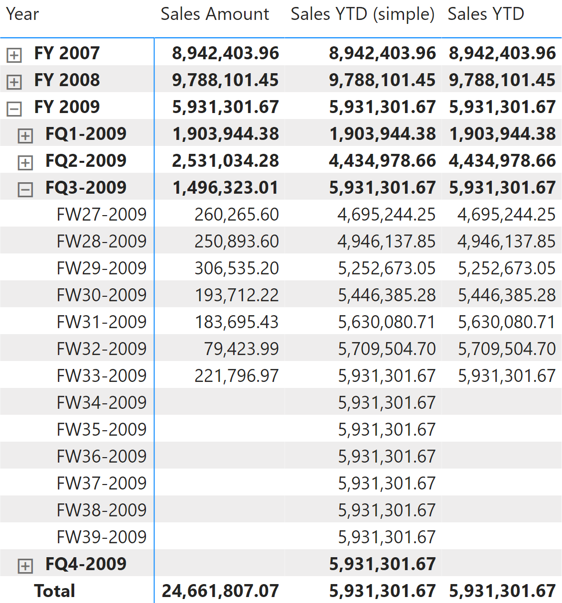
The measure filters all the days less than or equal to the last day visible in the last fiscal year. It also filters the last visible Fiscal Year Number:
Sales YTD (simple) :=
VAR LastDayAvailable = MAX ( 'Date'[Day of Fiscal Year Number] )
VAR LastFiscalYearAvailable = MAX ( 'Date'[Fiscal Year Number] )
VAR Result =
    CALCULATE (
        [Sales Amount],
        ALLEXCEPT ( 'Date', 'Date'[Working Day], 'Date'[Day of Week] ),
        'Date'[Day of Fiscal Year Number] <= LastDayAvailable,
        'Date'[Fiscal Year Number] = LastFiscalYearAvailable
    )
RETURN
    Result
Because LastDayAvailable contains the last date visible in the filter context, Sales YTD (simple) shows data even for future dates in the year. We can avoid this behavior in the Sales YTD measure by returning a result only when ShowValueForDates returns TRUE:
Sales YTD :=
IF (
    [ShowValueForDates],
    VAR LastDayAvailable = MAX ( 'Date'[Day of Fiscal Year Number] )
    VAR LastFiscalYearAvailable = MAX ( 'Date'[Fiscal Year Number] )
    VAR Result =
        CALCULATE (
            [Sales Amount],
            ALLEXCEPT ( 'Date', 'Date'[Working Day], 'Date'[Day of Week] ),
            'Date'[Day of Fiscal Year Number] <= LastDayAvailable,
            'Date'[Fiscal Year Number] = LastFiscalYearAvailable
        )
    RETURN
        Result
)
ALLEXCEPT is required to preserve the filter-keep columns Working Day or Day of Week in case they are used in the report. To demonstrate this, we purposely created an incorrect measure: Sales YTD (wrong), which removes the filters from the Date table by using REMOVEFILTERS instead of ALLEXCEPT. By doing this, the formula loses the filter on Working Day used in the columns of the matrix, thus producing an incorrect result:
Sales YTD (wrong) :=
IF (
    [ShowValueForDates],
    VAR LastDayAvailable = MAX ( 'Date'[Day of Fiscal Year Number] )
    VAR LastFiscalYearAvailable = MAX ( 'Date'[Fiscal Year Number] )
    RETURN
        CALCULATE (
            [Sales Amount],
            REMOVEFILTERS ( 'Date' ),
            'Date'[Day of Fiscal Year Number] <= LastDayAvailable,
            'Date'[Fiscal Year Number] = LastFiscalYearAvailable
        )
)
Figure 2 shows the comparison of the correct and incorrect measures.
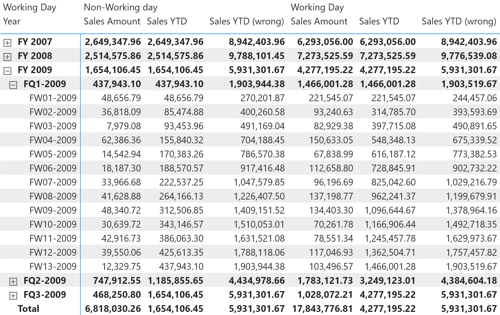
The Sales YTD (wrong) measure would work well if the Date table did not contain any filter-keep columns. The presence of filter-keep columns requires using ALLEXCEPT instead of REMOVEFILTERS. We used Sales YTD as an example, but the same concept is valid for all the other measures in this pattern.
Quarter-to-date total
Quarter-to-date aggregates data from the first day of the fiscal quarter, as shown in Figure 3.
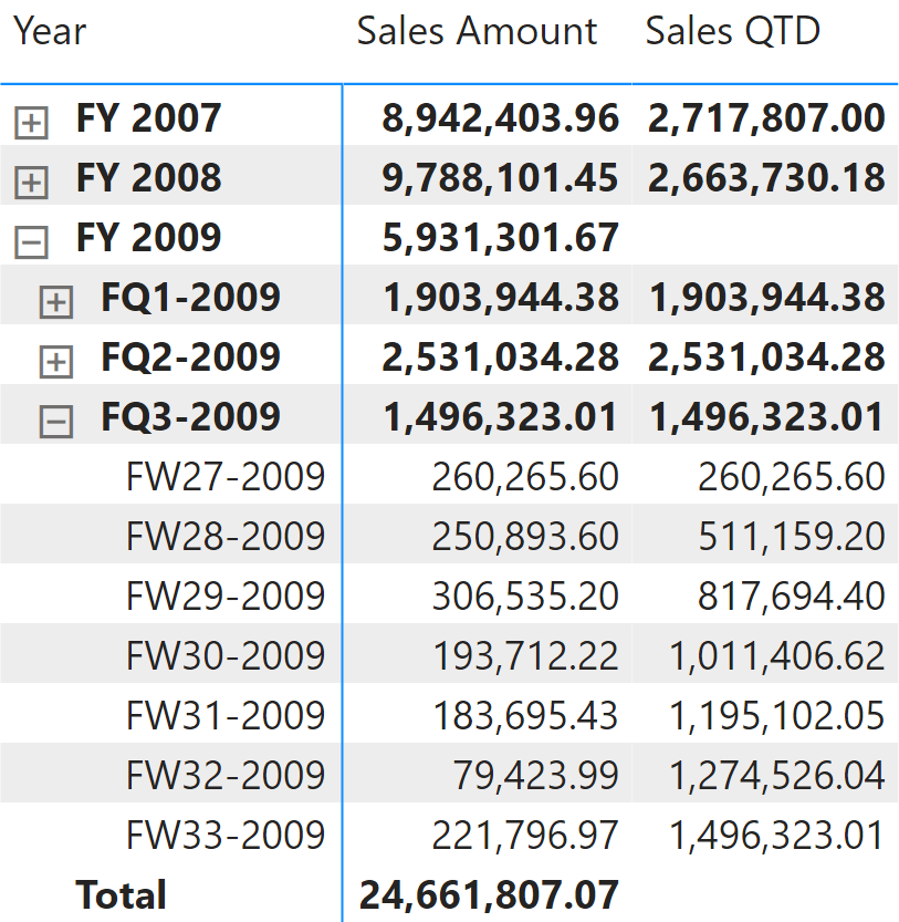
Quarter-to-date is computed with the same technique as the one we used for the year-to-date total. The only differences are the filters on Fiscal Year Quarter Number instead of Fiscal Year Number, and Day of Fiscal Quarter Number instead of Day of Fiscal Year Number.
Sales QTD :=
IF (
    [ShowValueForDates],
    VAR LastDayAvailable =  MAX ( 'Date'[Day of Fiscal Quarter Number] )
    VAR LastFiscalYearQuarterAvailable = MAX ( 'Date'[Fiscal Year Quarter Number] )
    VAR Result =
        CALCULATE (
            [Sales Amount],
            ALLEXCEPT ( 'Date', 'Date'[Working Day], 'Date'[Day of Week] ),
            'Date'[Day of Fiscal Quarter Number] <= LastDayAvailable,
            'Date'[Fiscal Year Quarter Number] = LastFiscalYearQuarterAvailable
        )
    RETURN
        Result
)
Month-to-date total
Month-to-date aggregates data starting from the first day of the fiscal month, as shown in Figure 4.
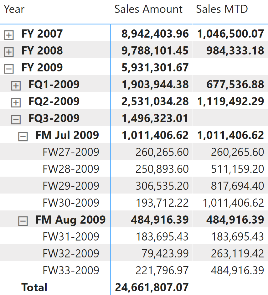
The month-to-date total is computed with a technique similar to those used in year-to-date total and quarter-to-date total, which filter all the days that are less than or equal to the last day visible in the last fiscal month. The filters are applied to the Day of Month Number and Year Month Number columns:
Sales MTD :=
IF (
    [ShowValueForDates],
    VAR LastDayAvailable =  MAX ( 'Date'[Day of Fiscal Month Number] )
    VAR LastFiscalYearMonthAvailable = MAX ( 'Date'[Fiscal Year Month Number] )
    VAR Result =
        CALCULATE (
            [Sales Amount],
            ALLEXCEPT ( 'Date', 'Date'[Working Day], 'Date'[Day of Week] ),
            'Date'[Day of Fiscal Month Number] <= LastDayAvailable,
            'Date'[Fiscal Year Month Number] = LastFiscalYearMonthAvailable
        )
    RETURN
        Result
)
The measure filters Day of Fiscal Month Number instead of Day of Fiscal Year Number. The reason is to filter a column with a lower number of unique values, which is a best practice from a query performance standpoint.
Week-to-date total
Week-to-date aggregates data from the first day of the week, as shown in Figure 5.
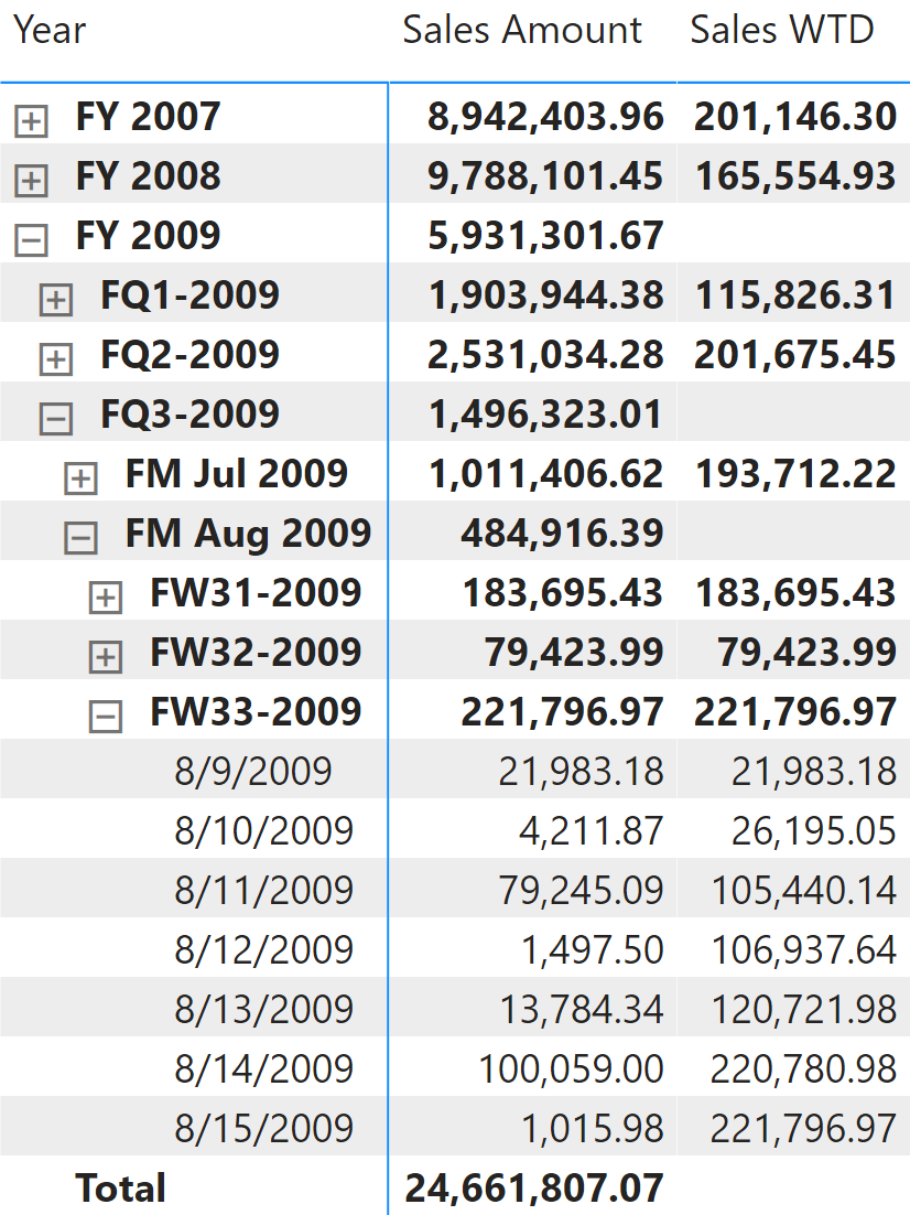
The week-to-date total is computed with a technique similar to those used in year-to-date total and quarter-to-date total, which filters all the days that are less than or equal to the last weekday day number visible in the last fiscal week. The filters are applied to the Day of Week Number and Fiscal Year Week Number columns:
Sales WTD :=
IF (
    [ShowValueForDates],
    VAR LastDayOfWeekAvailable =  MAX ( 'Date'[Day of Week Number] )
    VAR LastFiscalYearWeekAvailable = MAX ( 'Date'[Fiscal Year Week Number] )
    VAR Result =
        CALCULATE (
            [Sales Amount],
            ALLEXCEPT ( 'Date', 'Date'[Working Day], 'Date'[Day of Week] ),
            'Date'[Day of Week Number] <= LastDayOfWeekAvailable,
            'Date'[Fiscal Year Week Number] = LastFiscalYearWeekAvailable
        )
    RETURN
        Result
)
The measure filters Day of Week Number instead of Day of Fiscal Year Number. This is to filter a column with a lower number of unique values, which is a best practice from a query performance standpoint.
Computing period-over-period growth
A common requirement is to compare a time period with the same time period in the previous year, quarter, or week. We do not look at the comparison over the previous month because in a 4-4-5 calendar there may be a different number of weeks within the months. In order to achieve a fair comparison, the measure should work with an equivalent period, also taking into account that the last week/quarter/year could be incomplete. For these reasons, the calculations shown in this section use the Date[DateWithSales] calculated column, as described in the article, Hiding future dates for calculations in DAX.
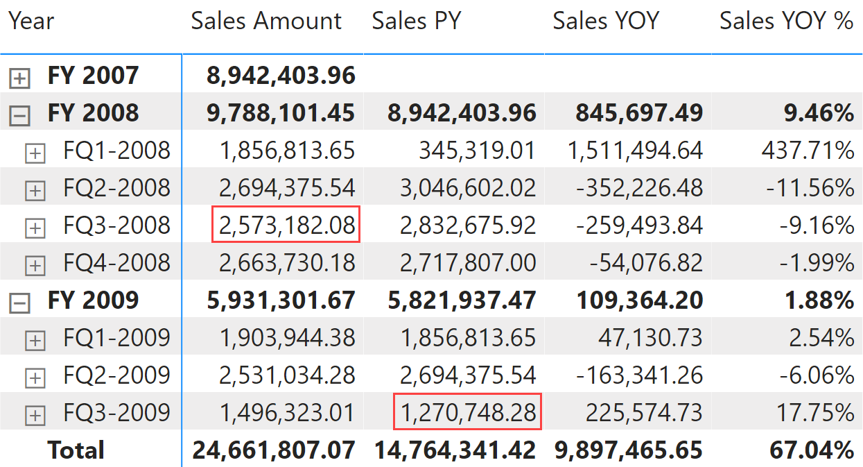
Year-over-year growth
Year-over-year compares a time period to the equivalent time period in the previous year. In this example, data is available until August 15, 2009. For this reason, Sales PY shows numbers related to FY 2009 and takes into account only transactions before August 15, 2008. Figure 6 shows that Sales Amount of FQ3-2008 is 2,573,182.08, whereas Sales PY for FQ3-2009 returns 1,270,748.28 because the measure considers only sales up to August 15, 2008.
Sales PY uses a standard technique that shifts the selection by the number of months defined in the MonthsOffset variable. In Sales PY the variable is set to 12, to move back in time by 12 months. The next measures, Sales PQ and Sales PM, use the same code. The only difference is the value assigned to MonthsOffset.
Sales PY iterates every year active in the filter context. For each year, it retrieves the days selected in the year while ignoring the filter-keep columns (Working Day, Day of Week and Day of Week Number in our example). The days are evaluated using the relative day number within the year. These days are applied as a filter on the previous year. The filters over filter-keep columns are kept in the filter context by using ALLEXCEPT:
Sales PY :=
IF (
    [ShowValueForDates],
    SUMX (
        VALUES ( 'Date'[Fiscal Year Number] ),
        VAR CurrentFiscalYearNumber = 'Date'[Fiscal Year Number]
        VAR DaysSelected =
            CALCULATETABLE (
                VALUES ( 'Date'[Day of Fiscal Year Number] ),
                REMOVEFILTERS (
                    'Date'[Working Day],
                    'Date'[Day of Week],
                    'Date'[Day of Week Number]
                ),
                'Date'[DateWithSales] = TRUE
            )
        RETURN
            CALCULATE (
                [Sales Amount],
                'Date'[Fiscal Year Number] = CurrentFiscalYearNumber - 1,
                DaysSelected,
                ALLEXCEPT ( 'Date', 'Date'[Working Day], 'Date'[Day of Week] )
            )
    )
)
The year-over-year growth is computed as an amount in Sales YOY and as a percentage in Sales YOY %. Both measures use Sales PY to take into account only dates up to August 15, 2009:
Sales YOY :=
VAR ValueCurrentPeriod = [Sales Amount]
VAR ValuePreviousPeriod = [Sales PY]
VAR Result =
    IF (
        NOT ISBLANK ( ValueCurrentPeriod )
            && NOT ISBLANK ( ValuePreviousPeriod ),
        ValueCurrentPeriod - ValuePreviousPeriod
    )
RETURN
    Result
Sales YOY % :=
DIVIDE (
    [Sales YOY],
    [Sales PY]
)
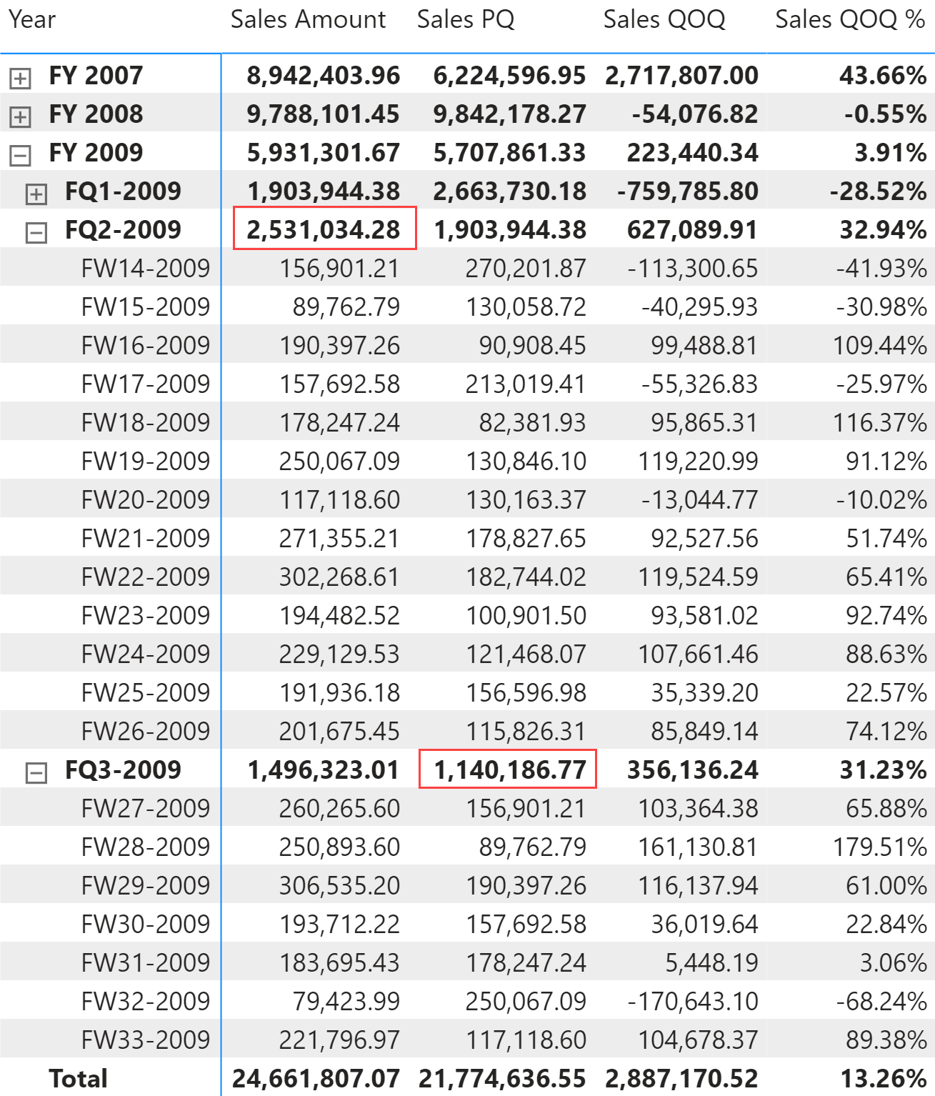
Quarter-over-quarter growth
Quarter-over-quarter compares a time period with the equivalent time period in the previous quarter. In this example, data is available until August 15, 2009, which is more than half of the third quarter of FY 2009 – it is day 49 in that quarter. Therefore, Sales PQ for August 2009 – the second month of the third quarter – shows sales until May 16, 2009, which is day 49 in the previous quarter, FQ2-2009. Figure 7 shows that Sales Amount of FQ2-2009 is 2,531,034.28, whereas Sales PQ for FQ3-2009 returns 1,140,186.77, restricted to sales performed up to May 16, 2009.
Sales PQ uses the technique described for Sales PY. The only difference is that instead of iterating Fiscal Year Number, it iterates Fiscal Year Quarter Number and applies the filter over Day of Fiscal Quarter Number instead of over Day of Fiscal Year Number:
Sales PQ :=
IF (
    [ShowValueForDates],
    SUMX (
        VALUES ( 'Date'[Fiscal Year Quarter Number] ),
        VAR CurrentFiscalYearQuarterNumber = 'Date'[Fiscal Year Quarter Number]
        VAR DaysSelected =
            CALCULATETABLE (
                VALUES ( 'Date'[Day of Fiscal Quarter Number] ),
                REMOVEFILTERS (
                    'Date'[Working Day],
                    'Date'[Day of Week],
                    'Date'[Day of Week Number]
                ),
                'Date'[DateWithSales] = TRUE
            )
        RETURN
            CALCULATE (
                [Sales Amount],
                'Date'[Fiscal Year Quarter Number] = CurrentFiscalYearQuarterNumber - 1,
                DaysSelected,
                ALLEXCEPT ( 'Date', 'Date'[Working Day], 'Date'[Day of Week] )
            )
    )
)
The quarter-over-quarter growth is computed as an amount in Sales QOQ and as a percentage in Sales QOQ %. Both measures use Sales PQ to guarantee a fair comparison:
Sales QOQ :=
VAR ValueCurrentPeriod = [Sales Amount]
VAR ValuePreviousPeriod = [Sales PQ]
VAR Result =
    IF (
        NOT ISBLANK ( ValueCurrentPeriod ) && NOT ISBLANK ( ValuePreviousPeriod ),
        ValueCurrentPeriod - ValuePreviousPeriod
    )
RETURN
    Result
Sales QOQ % :=
DIVIDE (
    [Sales QOQ],
    [Sales PQ]
)
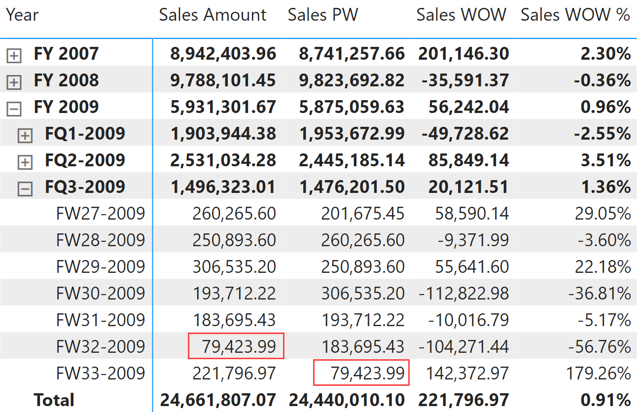
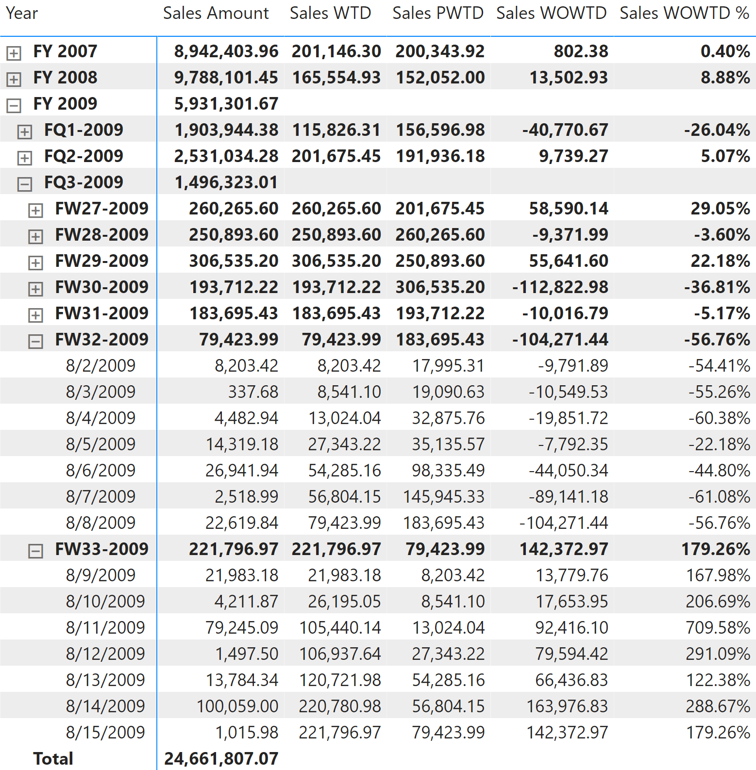
Week-over-week growth
Week-over-week compares a time period with its equivalent in the previous week. The calculation is similar to year-over-year and quarter-over-quarter growth, even though the data available does not show a specific example of a partial week corresponding to the last day available (August 15, 2019). The Sales PW measure sums all the weeks of the period shifted back by one week if the report aggregates more weeks, like at the year and quarter level. Figure 8 shows an example of the result.
Sales PW uses the technique described for Sales PY. The only difference is that instead of iterating Fiscal Year Number, it iterates Fiscal Year Week Number and applies the filter over Day of Week Number instead of over Day of Fiscal Year Number:
Sales PW :=
IF (
    [ShowValueForDates],
    SUMX (
        VALUES ( 'Date'[Fiscal Year Week Number] ),
        VAR CurrentFiscalYearWeekNumber = 'Date'[Fiscal Year Week Number]
        VAR DaysSelected =
            CALCULATETABLE (
                VALUES ( 'Date'[Day of Week Number] ),
                REMOVEFILTERS (
                    'Date'[Working Day],
                    'Date'[Day of Week],
                    'Date'[Day of Week Number]
                ),
                'Date'[DateWithSales] = TRUE
            )
        RETURN
            CALCULATE (
                [Sales Amount],
                'Date'[Fiscal Year Week Number] = CurrentFiscalYearWeekNumber - 1,
                KEEPFILTERS ( DaysSelected ),
                ALLEXCEPT ( 'Date', 'Date'[Working Day], 'Date'[Day of Week] )
            )
    )
)
The week-over-week growth is computed as an amount in Sales WOW and as a percentage in Sales WOW %. Both measures use Sales PW to guarantee a fair comparison:
Sales WOW :=
VAR ValueCurrentPeriod = [Sales Amount]
VAR ValuePreviousPeriod = [Sales PW]
VAR Result =
    IF (
        NOT ISBLANK ( ValueCurrentPeriod ) && NOT ISBLANK ( ValuePreviousPeriod ),
        ValueCurrentPeriod - ValuePreviousPeriod
    )
RETURN
    Result
Sales WOW % :=
DIVIDE (
    [Sales WOW],
    [Sales PW]
)
Period-over-period growth
Period-over-period growth automatically selects one of the measures described earlier in this section based on the current selection of the visualization. For example, it returns the value of week-over-week growth measures if the visualization displays data at the week level, and switches to quarter-over-quarter or year-over-year growth measures if the visualization shows the total at the quarter or year level, respectively. The month level is not supported on a 4-4-5 calendar. The expected result is visible in Figure 9.
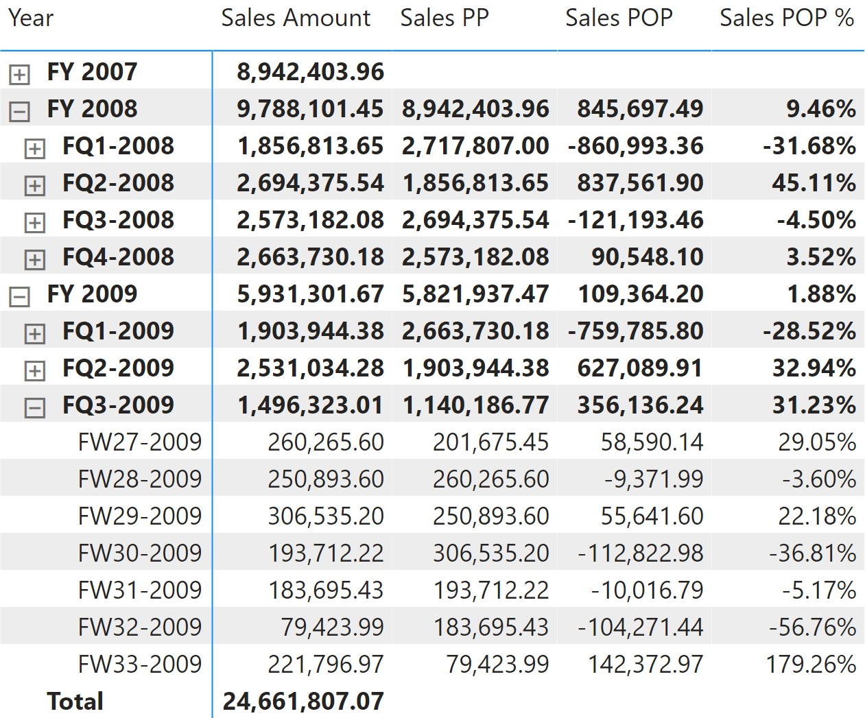
The three measures Sales PP, Sales POP, and Sales POP % redirect the evaluation to the corresponding year, quarter, and week measures depending on the level selected in the report. ISINSCOPE detects the level used in the report. The arguments passed to ISINSCOPE are the attributes used in the rows of the Matrix visual in Figure 9. The measures are defined as follows:
Sales POP % :=
SWITCH (
    TRUE,
    ISINSCOPE ( 'Date'[Fiscal Year Week] ), [Sales WOW %],
    -- The month level should not be managed in a 445 calendar
    ISINSCOPE ( 'Date'[Fiscal Year Quarter] ), [Sales QOQ %],
    ISINSCOPE ( 'Date'[Fiscal Year] ), [Sales YOY %]
)
Sales POP :=
SWITCH (
    TRUE,
    ISINSCOPE ( 'Date'[Fiscal Year Week] ), [Sales WOW],
    -- The month level should not be managed in a 445 calendar
    ISINSCOPE ( 'Date'[Fiscal Year Quarter] ), [Sales QOQ],
    ISINSCOPE ( 'Date'[Fiscal Year] ), [Sales YOY]
)
Sales PP :=
SWITCH (
    TRUE,
    ISINSCOPE ( 'Date'[Fiscal Year Week] ), [Sales PW],
    -- The month level should not be managed in a 445 calendar
    ISINSCOPE ( 'Date'[Fiscal Year Quarter] ), [Sales PQ],
    ISINSCOPE ( 'Date'[Fiscal Year] ), [Sales PY]
)
Computing period-to-date growth
The growth of a “to-date” measure is the comparison of the “to-date” measure with the same measure over an equivalent time period with a specific offset. For example, you can compare a year-to-date aggregation against the year-to-date in the previous fiscal year, that is with an offset of one fiscal year.
All the measures in this set of calculations take care of partial periods. Because data is available only until August 15, 2009 in our example, the measures make sure the previous year does not report dates after August 15, 2008.
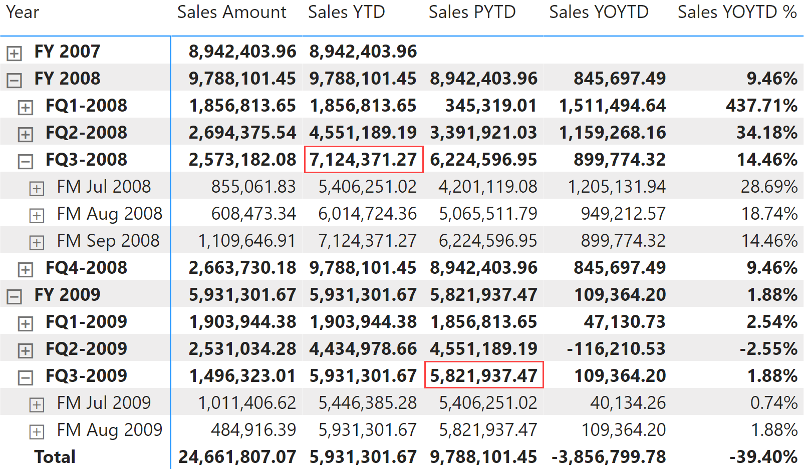
Year-over-year-to-date growth
Year-over-year-to-date growth compares the year-to-date on a specific date with the year-to-date on an equivalent date in the previous year. Figure 10 shows that Sales PYTD in FY 2009 is considering only sales until August 16, 2008, because it is the same relative day within FY 2008 as is August 15, 2009 for FY 2009. For this reason, Sales YTD of FQ3-2008 is 7,124,371.27, whereas Sales PYTD for FQ3-2009 is less: 5,821,937.47.
Sales PYTD is like Sales YTD: it filters the previous value in Fiscal Year Number instead of the last year visible in the filter context. The main difference is the evaluation of LastDayOfFiscalYearAvailable, which must consider only dates with sales while ignoring the filter on filter-keep columns, which are considered in the evaluation of Sales Amount:
Sales PYTD :=
IF (
    [ShowValueForDates],
    VAR PreviousFiscalYear = MAX ( 'Date'[Fiscal Year Number] ) - 1
    VAR LastDayOfFiscalYearAvailable =
        CALCULATE (
            MAX ( 'Date'[Day of Fiscal Year Number] ),
            REMOVEFILTERS (                -- Remove filters from
                'Date'[Working Day],       -- filter-keep columns
                'Date'[Day of Week],       -- to get the last day with data
                'Date'[Day of Week Number] -- selected in the report
            ),
            'Date'[DateWithSales] = TRUE
        )
    VAR Result =
        CALCULATE (
            [Sales Amount],
            ALLEXCEPT ( 'Date', 'Date'[Working Day], 'Date'[Day of Week] ),
            'Date'[Fiscal Year Number] = PreviousFiscalYear,
            'Date'[Day of Fiscal Year Number] <= LastDayOfFiscalYearAvailable,
            'Date'[DateWithSales] = TRUE
        )
    RETURN
        Result
)
Sales YOYTD and Sales YOYTD % rely on Sales PYTD to guarantee a fair comparison:
Sales YOYTD :=
VAR ValueCurrentPeriod = [Sales YTD]
VAR ValuePreviousPeriod = [Sales PYTD]
VAR Result =
    IF (
        NOT ISBLANK ( ValueCurrentPeriod ) && NOT ISBLANK ( ValuePreviousPeriod ),
        ValueCurrentPeriod - ValuePreviousPeriod
    )
RETURN
    Result
Sales YOYTD % :=
DIVIDE (
    [Sales YOYTD],
    [Sales PYTD]
)
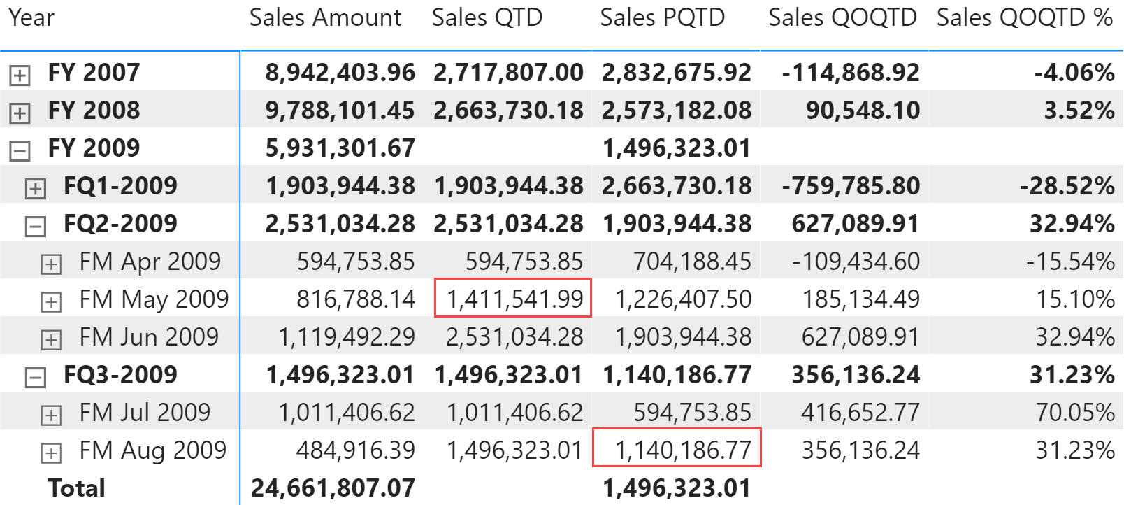
Quarter-over-quarter-to-date growth
Quarter-over-quarter-to-date growth compares the quarter-to-date on a specific date with the quarter-to-date on an equivalent date in the previous quarter. Figure 11 shows that Sales PQTD in FW August 2009 is considering only transactions that occurred prior to May 16, 2009, to get the corresponding part of the previous quarter. For this reason Sales QTD of FW May 2009 is 1,411,541.99, whereas Sales PQTD for FW August 2009 is lower: 1,140,186.77.
Sales PQTD is like Sales QTD; it filters the previous value in Fiscal Year Quarter Number instead of the last quarter visible in the filter context. The main difference is the evaluation of LastDayOfFiscalYearQuarterAvailable, which must consider only dates with sales while ignoring the filter on filter-keep columns, which are considered in the evaluation of Sales Amount:
Sales PQTD :=
IF (
    [ShowValueForDates],
    VAR PreviousFiscalYearQuarter = MAX ( 'Date'[Fiscal Year Quarter Number] ) - 1
    VAR LastDayOfFiscalYearQuarterAvailable =
        CALCULATE (
            MAX ( 'Date'[Day of Fiscal Quarter Number] ),
            REMOVEFILTERS (                -- Remove filters from
                'Date'[Working Day],       -- filter-keep columns
                'Date'[Day of Week],       -- to get the last day with data
                'Date'[Day of Week Number] -- selected in the report
            ),
            'Date'[DateWithSales] = TRUE
        )
    VAR Result =
        CALCULATE (
            [Sales Amount],
            ALLEXCEPT ( 'Date', 'Date'[Working Day], 'Date'[Day of Week] ),
            'Date'[Fiscal Year Quarter Number] = PreviousFiscalYearQuarter,
            'Date'[Day of Fiscal Quarter Number] <= LastDayOfFiscalYearQuarterAvailable,
            'Date'[DateWithSales] = TRUE
        )
    RETURN
        Result
)
Sales QOQTD and Sales QOQTD % rely on Sales PQTD to guarantee a fair comparison:
Sales QOQTD :=
VAR ValueCurrentPeriod = [Sales QTD]
VAR ValuePreviousPeriod = [Sales PQTD]
VAR Result =
    IF (
        NOT ISBLANK ( ValueCurrentPeriod ) && NOT ISBLANK ( ValuePreviousPeriod ),
        ValueCurrentPeriod - ValuePreviousPeriod
    )
RETURN
    Result
Sales QOQTD % :=
DIVIDE (
    [Sales QOQTD],
    [Sales PQTD]
)
Week-over-week-to-date growth
Week-over-week-to-date growth compares a week-to-date on a specific date with the week-to-date on an equivalent date in the previous week. The calculation is similar to year-over-year and quarter-over-quarter growth, even though the data available does not show a specific example of a partial week corresponding to the last day available (August 15, 2019). Figure 12 shows an example of the result.
Sales PWTD is like Sales WTD; it filters the previous value in Fiscal Year Week Number instead of the last week visible in the filter context. The main difference is the evaluation of LastDayOfFiscalYearWeekAvailable, which must consider only dates with sales while ignoring the filter on filter-keep columns, which are considered in the evaluation of Sales Amount:
Sales PWTD :=
IF (
    [ShowValueForDates],
    VAR PreviousFiscalYearWeek = MAX ( 'Date'[Fiscal Year Week Number] ) - 1
    VAR LastDayOfWeekAvailable =
        CALCULATE (
            MAX ( 'Date'[Day of Week Number] ),
            REMOVEFILTERS (                -- Remove filters from
                'Date'[Working Day],       -- filter-keep columns
                'Date'[Day of Week],       -- to get the last day with data
                'Date'[Day of Week Number] -- selected in the report
            ),
            'Date'[DateWithSales] = TRUE
        )
    VAR Result =
        CALCULATE (
            [Sales Amount],
            ALLEXCEPT ( 'Date', 'Date'[Working Day], 'Date'[Day of Week] ),
            'Date'[Fiscal Year Week Number] = PreviousFiscalYearWeek,
            'Date'[Day of Week Number] <= LastDayOfWeekAvailable,
            'Date'[DateWithSales] = TRUE
        )
    RETURN
        Result
)
Sales WOWTD and Sales WOWTD % rely on the Sales PWTD measure to guarantee a fair comparison:
Sales WOWTD :=
VAR ValueCurrentPeriod = [Sales WTD]
VAR ValuePreviousPeriod = [Sales PWTD]
VAR Result =
    IF (
        NOT ISBLANK ( ValueCurrentPeriod )
            && NOT ISBLANK ( ValuePreviousPeriod ),
        ValueCurrentPeriod - ValuePreviousPeriod
    )
RETURN
    Result
Sales WOWTD % :=
DIVIDE (
    [Sales WOWTD],
    [Sales PWTD]
)
Comparing period-to-date with previous full period
Comparing a to-date aggregation with the previous full period is useful when you consider the previous period as a benchmark. Once the current year-to-date reaches 100% of the full previous year, this means we have reached the same performance as the previous full period, hopefully in fewer days.
Year-to-date over the full previous year
Year-to-date over the full previous year compares the year-to-date against the entire previous year. Figure 13 shows that in FW48-2008 Sales YTD surpassed the value of Sales Amount for the entire fiscal year 2007. Sales YTDOPY % provides an immediate comparison of the year-to-date with the total of the previous fiscal year; it shows growth over the previous fiscal year when the percentage is positive.
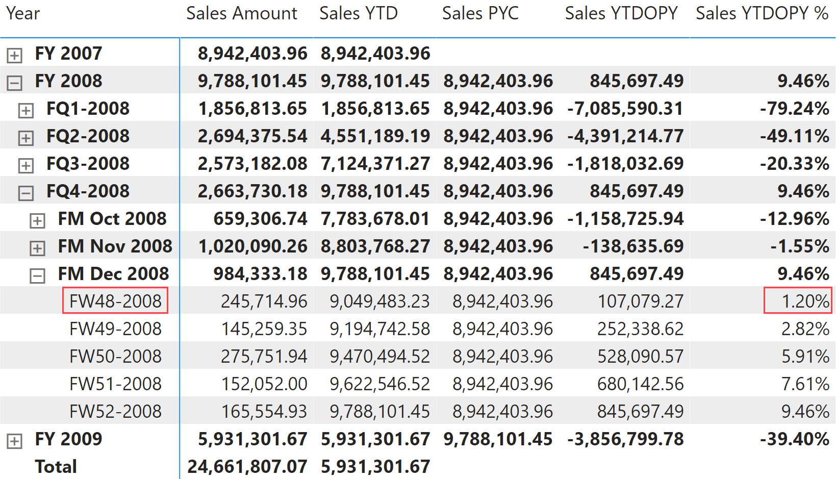
The year-to-date-over-previous-year growth is computed by the Sales YTDOPY and Sales YTDOPY % measures; these rely on the Sales YTD measure to compute the year-to-date value, and on the Sales PYC measure to get the sales amount of the entire previous fiscal year:
Sales PYC :=
IF (
    [ShowValueForDates] && HASONEVALUE ( 'Date'[Fiscal Year Number] ),
    VAR PreviousFiscalYear = MAX ( 'Date'[Fiscal Year Number] ) - 1
    VAR Result =
        CALCULATE (
            [Sales Amount],
            ALLEXCEPT ( 'Date', 'Date'[Working Day], 'Date'[Day of Week] ),
            'Date'[Fiscal Year Number] = PreviousFiscalYear
        )
    RETURN
        Result
)
Sales YTDOPY :=
VAR ValueCurrentPeriod = [Sales YTD]
VAR ValuePreviousPeriod = [Sales PYC]
VAR Result =
    IF (
        NOT ISBLANK ( ValueCurrentPeriod ) && NOT ISBLANK ( ValuePreviousPeriod ),
        ValueCurrentPeriod - ValuePreviousPeriod
    )
RETURN
    Result
Sales YTDOPY % :=
DIVIDE (
    [Sales YTDOPY],
    [Sales PYC]
)
Quarter-to-date over the full previous quarter
Quarter-to-date over the full previous quarter compares the quarter-to-date against the entire previous fiscal quarter. Figure 14 shows that Sales QTD surpassed the total Sales Amount for FQ1-2009 in FW23-2009. Sales QTDOPQ % provides an immediate comparison of the quarter-to-date with the total of the previous quarter; it shows growth over the previous quarter when the percentage is positive.
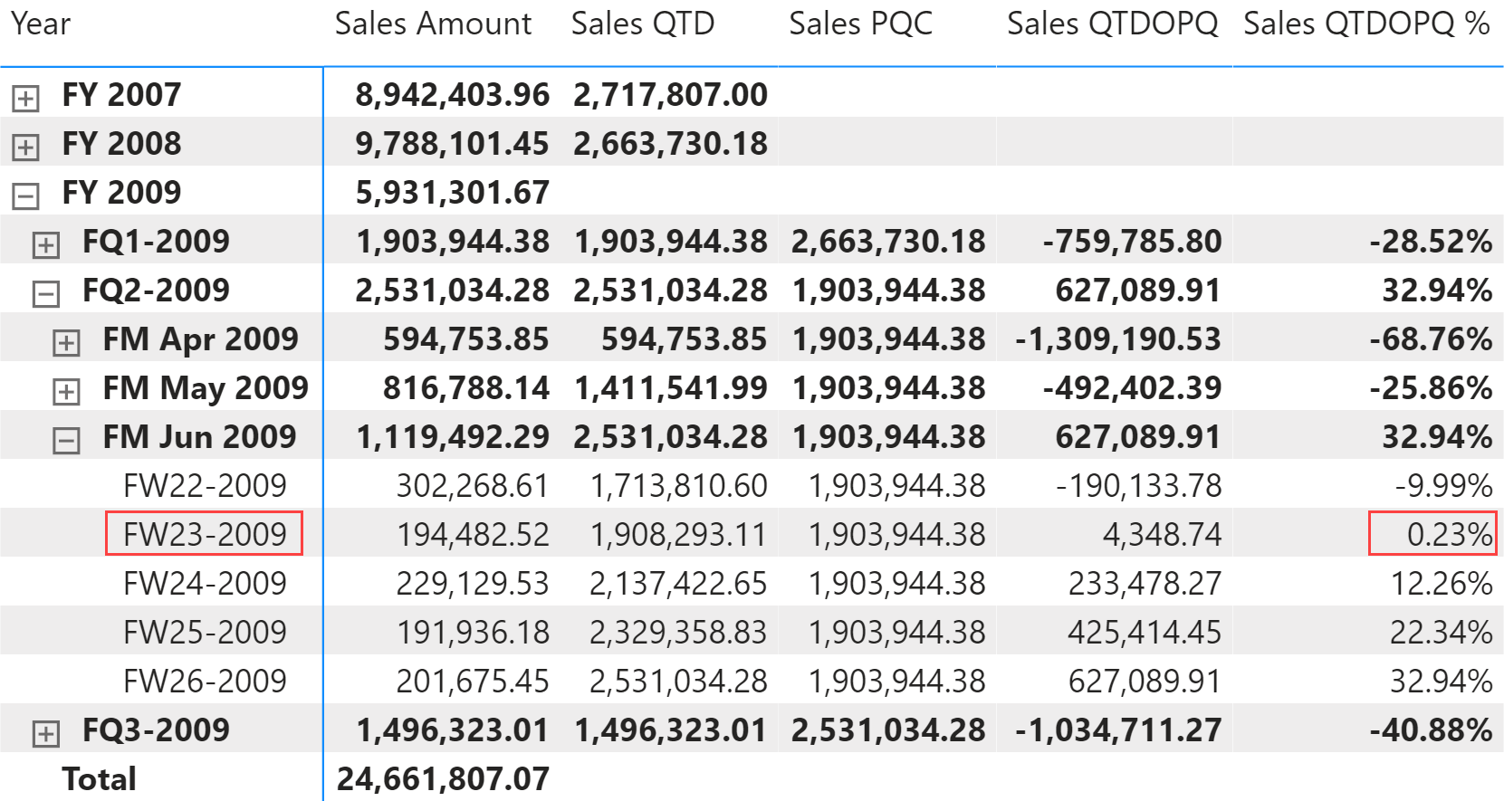
The quarter-to-date-over-previous-quarter growth is computed with the Sales QTDOPQ and Sales QTDOPQ % measures. These rely on the Sales QTD measure to compute the quarter-to-date value, and on the Sales PQC measure to get the sales amount of the entire previous quarter:
Sales PQC :=
IF (
    [ShowValueForDates] && HASONEVALUE ( 'Date'[Fiscal Year Quarter Number] ),
    VAR PreviousFiscalYearQuarter = MAX ( 'Date'[Fiscal Year Quarter Number] ) - 1
    VAR Result =
        CALCULATE (
            [Sales Amount],
            ALLEXCEPT ( 'Date', 'Date'[Working Day], 'Date'[Day of Week] ),
            'Date'[Fiscal Year Quarter Number] = PreviousFiscalYearQuarter
        )
    RETURN
        Result
)
Sales QTDOPQ :=
VAR ValueCurrentPeriod = [Sales QTD]
VAR ValuePreviousPeriod = [Sales PQC]
VAR Result =
    IF (
        NOT ISBLANK ( ValueCurrentPeriod ) && NOT ISBLANK ( ValuePreviousPeriod ),
        ValueCurrentPeriod - ValuePreviousPeriod
    )
RETURN
    Result
Sales QTDOPQ % :=
DIVIDE (
    [Sales QTDOPQ],
    [Sales PQC]
)
Week-to-date over the full previous week
The week-to-date over the full previous week compares the week-to-date against the entire previous week. Figure 15 shows that Sales WTD during FW33-2009 surpasses the total Sales Amount for FW32-2009. Sales WTDOPW% provides an immediate comparison of the week-to-date with the total of the previous week; it shows growth over the previous week when the percentage is positive, as is the case starting from August 11, 2009.
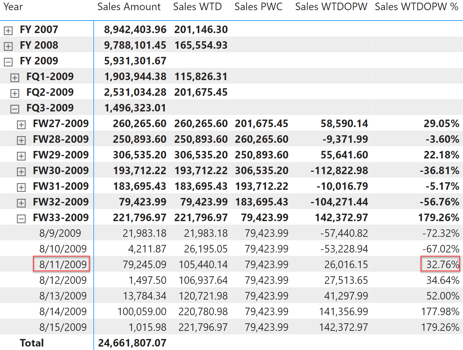
The week-to-date-over-previous-week growth is computed with the Sales WTDOPW % and Sales WTDOPW measures. These rely on the Sales WTD measure to compute the week-to-date value, and on the Sales PWC measure to get the sales amount of the entire previous week:
Sales PWC :=
IF (
    [ShowValueForDates] && HASONEVALUE ( 'Date'[Fiscal Year Week Number] ),
    VAR PreviousFiscalYearWeek = MAX ( 'Date'[Fiscal Year Week Number] ) - 1
    VAR Result =
        CALCULATE (
            [Sales Amount],
            ALLEXCEPT ( 'Date', 'Date'[Working Day], 'Date'[Day of Week] ),
            'Date'[Fiscal Year Week Number] = PreviousFiscalYearWeek
        )
    RETURN
        Result
)
Sales WTDOPW :=
VAR ValueCurrentPeriod = [Sales WTD]
VAR ValuePreviousPeriod = [Sales PWC]
VAR Result =
    IF (
        NOT ISBLANK ( ValueCurrentPeriod ) && NOT ISBLANK ( ValuePreviousPeriod ),
        ValueCurrentPeriod - ValuePreviousPeriod
    )
RETURN
    Result
Sales WTDOPW % :=
DIVIDE (
    [Sales WTDOPW],
    [Sales PWC]
)
Using moving annual total calculations
A common way to aggregate data over several months is by using the moving annual total instead of the year-to-date. In the week-based calendar, the moving annual total includes the last 52 weeks (364 days) of data.
Moving annual total
Sales MAT (364) computes the moving annual total, as shown in Figure 16.
The Sales MAT (364) measure defines a range over the Date[Date] column that includes the days of one complete year from the last day in the filter context:
Sales MAT (364) :=
IF (
    [ShowValueForDates],
    VAR LastDayMAT =  MAX ( 'Date'[Sequential Day Number] )
    VAR FirstDayMAT = LastDayMAT - 363
    VAR Result =
        CALCULATE (
            [Sales Amount],
            ALLEXCEPT ( 'Date', 'Date'[Working Day], 'Date'[Day of Week] ),
            'Date'[Sequential Day Number] >= FirstDayMAT
                && 'Date'[Sequential Day Number] <= LastDayMAT
        )
    RETURN
        Result
)
The Sales MAT (364) does not correspond to a year total in case the year has more than 52 weeks, as is the case every 5-6 years in the 4-4-5 calendar. Yet, it is a better measure to evaluate trends over time because it always includes the same number of days and weeks.
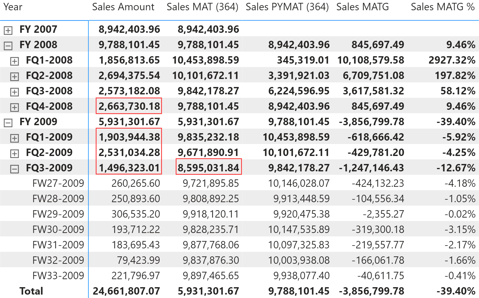
Moving annual total growth
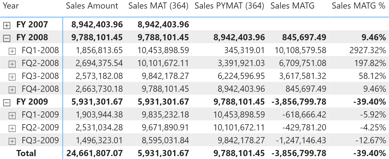
The moving annual total growth is computed with the Sales PYMAT (364), Sales MATG, and Sales MATG % measures, which rely on the Sales MAT (364) measure. Sales MAT (364) provides a correct value one year after the first sale ever, once it has collected one full year of data; it is not protected in case the current time period is shorter than a full year. For example, the amount for the fiscal year FY 2009 of Sales PYMAT (364) is 9,788,101.45, which corresponds to the Sales Amount of FY 2008 as shown in Figure 17. When compared with sales in FY 2009, this produces a comparison of less than 6 months – data being only available until August 15, 2009 – with a full fiscal year 2009. Similarly, you can see that Sales MATG % starts in FY 2008 with very high values and stabilizes after a year. This behavior is by design: the moving annual total is usually computed at the month or day granularity to show trends in a chart.
The measures are defined as follows:
Sales PYMAT (364) :=
IF (
    [ShowValueForDates],
    VAR LastDayAvailable = MAX ( 'Date'[Sequential Day Number] )
    VAR LastDayMAT = LastDayAvailable - 364 -- go back 52 weeks
    VAR FirstDayMAT = LastDayMAT - 363
    VAR Result =
        CALCULATE (
            [Sales Amount],
            ALLEXCEPT ( 'Date', 'Date'[Working Day], 'Date'[Day of Week] ),
            'Date'[Sequential Day Number] >= FirstDayMAT
                && 'Date'[Sequential Day Number] <= LastDayMAT
        )
    RETURN
        Result
)
Sales MATG :=
VAR ValueCurrentPeriod = [Sales MAT (364)]
VAR ValuePreviousPeriod = [Sales PYMAT (364)]
VAR Result =
    IF (
        NOT ISBLANK ( ValueCurrentPeriod ) && NOT ISBLANK ( ValuePreviousPeriod ),
        ValueCurrentPeriod - ValuePreviousPeriod
    )
RETURN
    Result
Sales MATG % :=
DIVIDE (
    [Sales MATG],
    [Sales PYMAT (364)]
)
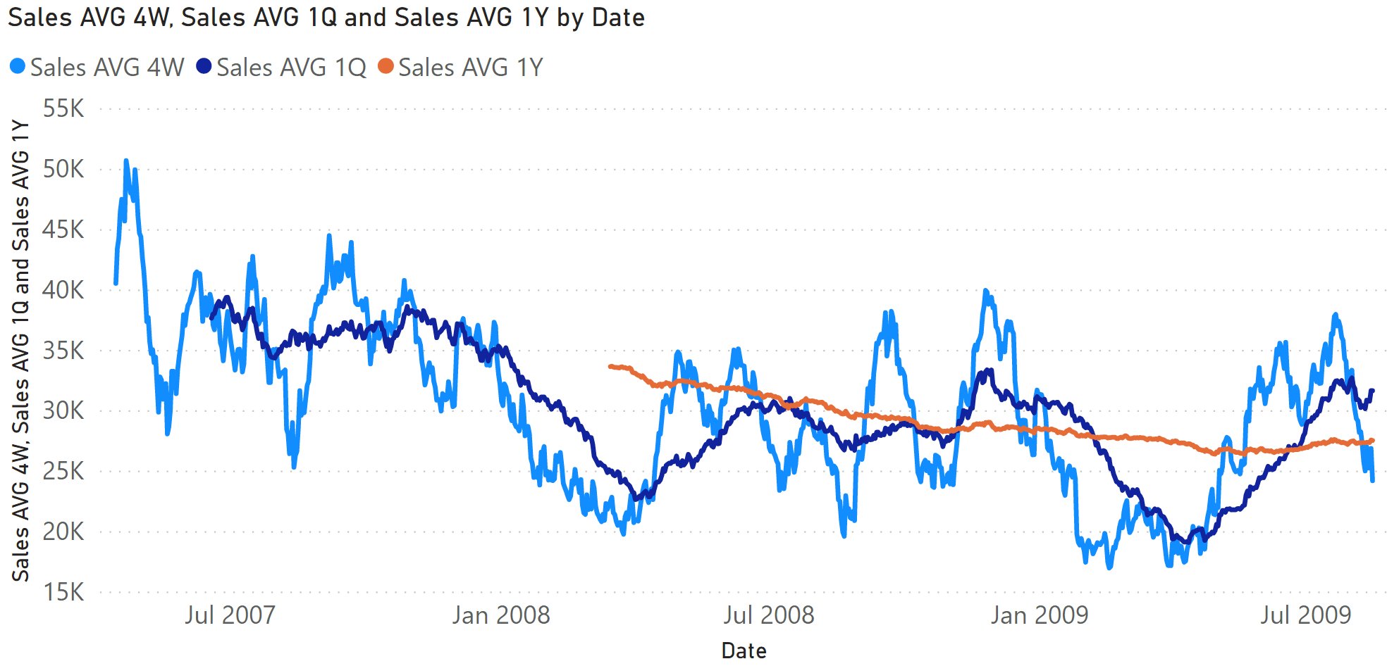
Moving averages
The moving average is typically used to display trends in line charts. Figure 18 includes the moving average of Sales Amount over four weeks (Sales AVG 4W), one quarter (Sales AVG 1Q), and a fiscal year (Sales AVG 1Y).
Moving average 4 weeks
The Sales AVG 4W measure computes the moving average over four weeks by iterating a list of the last 28 dates obtained in the Period4W variable. The Period4W variable retrieves the dates visible in the last 28 days with two exceptions; it ignores dates without sales, and it applies the filters existing on filter-keep columns in the Date table:
Sales AVG 4W :=
IF (
    [ShowValueForDates],
    VAR LastDayMAT =
        MAX ( 'Date'[Sequential Day Number] )
    VAR FirstDayMAT = LastDayMAT - 27
    VAR Period4W =
        CALCULATETABLE (
            VALUES ( 'Date'[Sequential Day Number] ),
            ALLEXCEPT (
                'Date',
                'Date'[Working Day],
                'Date'[Day of Week]
            ),
            'Date'[Sequential Day Number] >= FirstDayMAT
                && 'Date'[Sequential Day Number] <= LastDayMAT,
            'Date'[DateWithSales] = TRUE
        )
    VAR FirstDayWithData =
        CALCULATE (
            MIN ( Sales[Order Date] ),
            REMOVEFILTERS ()
        )
    VAR FirstDayInPeriod =
        MINX (
            Period4W,
            'Date'[Sequential Day Number]
        )
    VAR Result =
        IF (
            FirstDayWithData <= FirstDayInPeriod,
            CALCULATE (
                AVERAGEX ( Period4W, [Sales Amount] ),
                REMOVEFILTERS ( 'Date' )
            )
        )
    RETURN
        Result
)
This pattern is very flexible because it also works for non-additive measures. With that said, for a regular additive calculation Result can be implemented using a different and faster formula:
VAR Result =
    IF (
        FirstDayWithData <= FirstDayInPeriod,
        CALCULATE (
            DIVIDE (
                [Sales Amount],
                DISTINCTCOUNT ( Sales[Order Date] )
            ),
            REMOVEFILTERS ( 'Date' ),
            Period4W
        )
    )
Moving average 1 quarter
The Sales AVG 1Q measure computes the moving average over 13 weeks by iterating a list of the dates in the last quarter obtained in the Period1Q variable. The Period1Q variable retrieves the dates visible included in the last 13 weeks (91 days) with two exceptions; it ignores dates without sales, and it applies the filters existing on filter-keep columns in the Date table:
Sales AVG 1Q :=
IF (
    [ShowValueForDates],
    VAR LastDayMAT =
        MAX ( 'Date'[Sequential Day Number] )
    VAR FirstDayMAT = LastDayMAT - 13 * 7 + 1
    VAR Period1Q =
        CALCULATETABLE (
            VALUES ( 'Date'[Sequential Day Number] ),
            ALLEXCEPT ( 'Date', 'Date'[Working Day], 'Date'[Day of Week] ),
            'Date'[Sequential Day Number] >= FirstDayMAT
                && 'Date'[Sequential Day Number] <= LastDayMAT,
            'Date'[DateWithSales] = TRUE
        )
    VAR FirstDayWithData =
        CALCULATE (
            MIN ( Sales[Order Date] ),
            REMOVEFILTERS ()
        )
    VAR FirstDayInPeriod =
        MINX (
            Period1Q,
            'Date'[Sequential Day Number]
        )
    VAR Result =
        IF (
            FirstDayWithData <= FirstDayInPeriod,
            CALCULATE (
                AVERAGEX ( Period1Q, [Sales Amount] ),
                REMOVEFILTERS ( 'Date' )
            )
        )
    RETURN
        Result
)
For simple additive measures, the pattern based on DIVIDE which is shown for the moving average over four weeks (28 days) can also be used for the average over 91 days.
Moving average 1 year
The Sales AVG 1Y measure computes the moving average over one year by iterating a list of the dates in the last 364 days in the Period1Y variable. The Period1Y variable retrieves the dates visible included in the last fiscal year (only including 52 weeks) with two exceptions; it ignores dates without sales, and it applies the filters existing on filter-keep columns in the Date table:
Sales AVG 1Y :=
IF (
    [ShowValueForDates],
    VAR LastDayMAT =
        MAX ( 'Date'[Sequential Day Number] )
    VAR FirstDayMAT = LastDayMAT - 363
    VAR Period1Y =
        CALCULATETABLE (
            VALUES ( 'Date'[Sequential Day Number] ),
            ALLEXCEPT (
                'Date',
                'Date'[Working Day],
                'Date'[Day of Week]
            ),
            'Date'[Sequential Day Number] >= FirstDayMAT
                && 'Date'[Sequential Day Number] <= LastDayMAT,
            'Date'[DateWithSales] = TRUE
        )
    VAR FirstDayWithData =
        CALCULATE (
            MIN ( Sales[Order Date] ),
            REMOVEFILTERS ()
        )
    VAR FirstDayInPeriod =
        MINX (
            Period1Y,
            'Date'[Sequential Day Number]
        )
    VAR Result =
        IF (
            FirstDayWithData <= FirstDayInPeriod,
            CALCULATE (
                AVERAGEX ( Period1Y, [Sales Amount] ),
                REMOVEFILTERS ( 'Date' )
            )
        )
    RETURN
        Result
)
For simple additive measures, the pattern based on DIVIDE shown for the moving average over four weeks (28 days) can also be used for the average over 364 days.
Clear filters from the specified tables or columns.
REMOVEFILTERS ( [<TableNameOrColumnName>] [, <ColumnName> [, <ColumnName> [, … ] ] ] )
Returns all the rows in a table except for those rows that are affected by the specified column filters.
ALLEXCEPT ( <TableName>, <ColumnName> [, <ColumnName> [, … ] ] )
Returns true when the specified column is the level in a hierarchy of levels.
ISINSCOPE ( <ColumnName> )
Safe Divide function with ability to handle divide by zero case.
DIVIDE ( <Numerator>, <Denominator> [, <AlternateResult>] )
This pattern is included in the book DAX Patterns, Second Edition.


Video

Do you prefer a video?
This pattern is also available in video format. Take a peek at the preview, then unlock access to the full-length video on SQLBI.com.Watch the full video — 74 min.
Downloads
Download the sample files for Power BI / Excel 2016-2019: