Calculations reporting values at the start or the end of a time period are quite the challenge for any BI developer, and DAX is no exception. These measures are not hard to compute; the complicated part is understanding the desired behavior precisely. These calculations do not work by aggregating values throughout the entire period, as you would typically do for sales amounts. Instead, the calculations should return the value at the beginning or the end of a selected time period. These calculations are also known as semi-additive calculations. They are semi-additive because they do sum up specific attributes, like customers, but not over other attributes, like dates, all the while reporting the value at the beginning or end of the period.

As an example, we use a model that contains the current balance of bank accounts. Over the customers, the measure must be additive: the total balance for all customers is the sum of the balance for each customer. Nevertheless, when aggregating over time you cannot use the SUM function. The balance of a quarter is not the sum of individual monthly balances. Instead, the measure should report the last balance of the quarter.

There are many details that need to be addressed when defining the meaning of start or end of the period. This is the reason why this pattern contains many examples. We suggest you read all of them, so to better understand the subtle differences between the different examples before choosing the correct one for your specific scenario.

Introduction

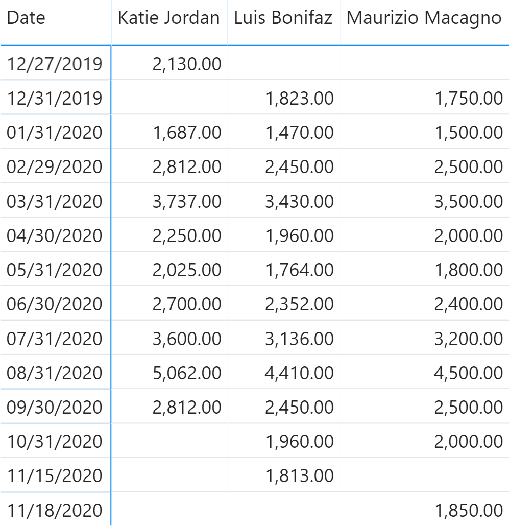
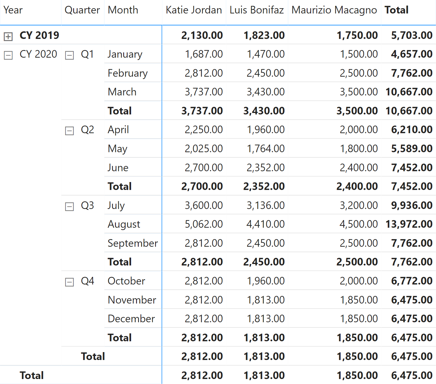
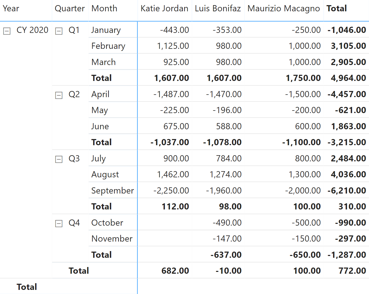
You have a model containing the balance of a few customers’ accounts. For each date, the number reported is the balance at that date. There are different reporting dates for different customers, as shown in Figure 1.

Because of the nature of the data, you cannot aggregate using SUM over time. Instead, you need to aggregate values at the month, quarter, and year level using the first or the last value of the period. Before looking at the code, you need to focus on some important details by answering the following questions:

What is the end balance of Katie Jordan’s account for 2020? Her last available balance is on September 30, so should we consider this to be the final value for 2020? Similarly, is the balance of Luis Bonifaz’s account zero or is it 1,813.00 at the end of 2020?
What is the total end balance over all three customers for 2020? Is it only the amount on Maurizio Macagno’s account – because his balance is the last one – or is it the sum of the last balance for each customer, at their respective dates?
What is the starting balance of 2020 for Luis Bonifaz? Is it the balance on January 1, 2020 or December 27/31, 2019?

As you see, there are multiple valid answers to each question, and none of them is more correct than the others. Depending on your requirements, you choose the pattern that best fits your needs. Indeed, all these patterns compute the balance at the start or the end of a period. The only and very relevant difference, is in the definition of what end of period means.

First and last date

The first and last date pattern is the simplest one. However, it can only be adopted in the few scenarios where the dataset always contains data at the beginning and at the end of each time period. The formula returns the balance using the first and last date of the Date table in the current filter context, regardless of whether data is present on the given date. If there is no balance on that date, its result is blank:

Measure in the Balances table

Balance LastDate :=
CALCULATE (
    SUM ( Balances[Balance] ),
    LASTDATE ( 'Date'[Date] )   -- Use FIRSTDATE for Balance FirstDate
)

This formula produces the result in Figure 2.

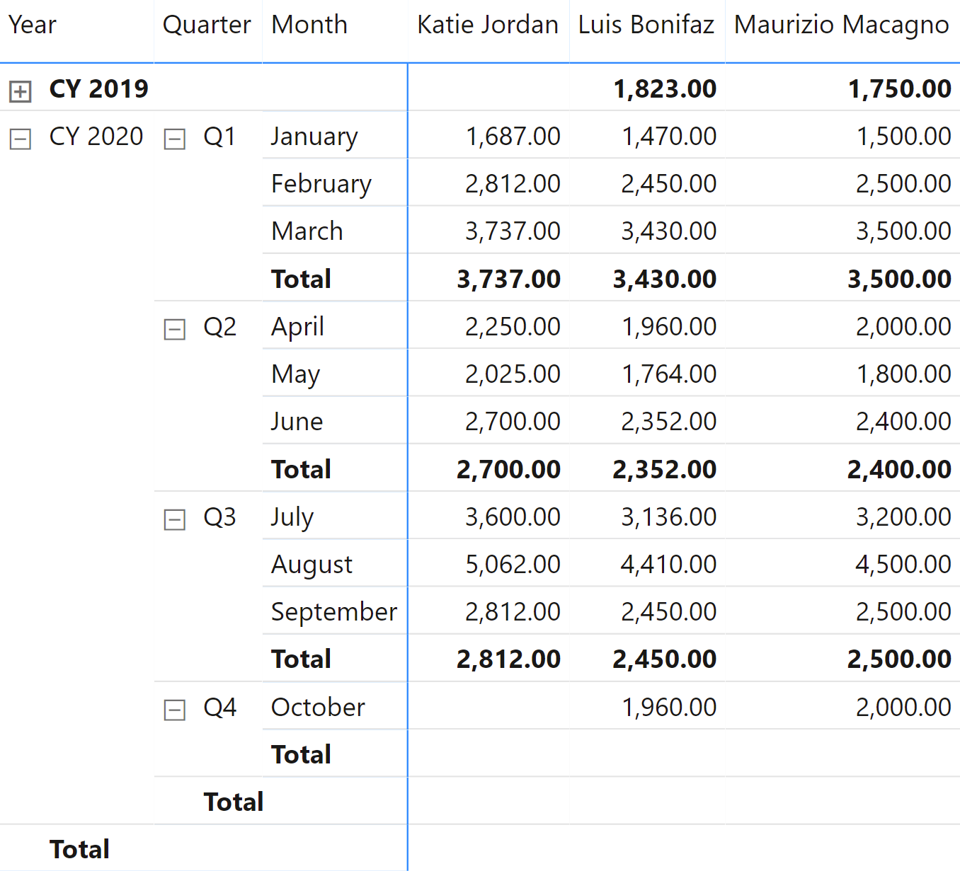
On months where data is not available on the last day of the month, the measure reports a blank. This pattern is the fastest among our many examples, but it only returns accurate results when data is stored on each and every day, or at least at the end of each and every time period. Therefore, it is the preferred pattern for example in financial applications where data is reported once every month.

First and last date with data

In this pattern, the formula searches the last date for which there is data in the current filter context. Therefore, instead of finding the last date in the Date table, it searches for the last date in the Balances table. The result is visible in Figure 3.

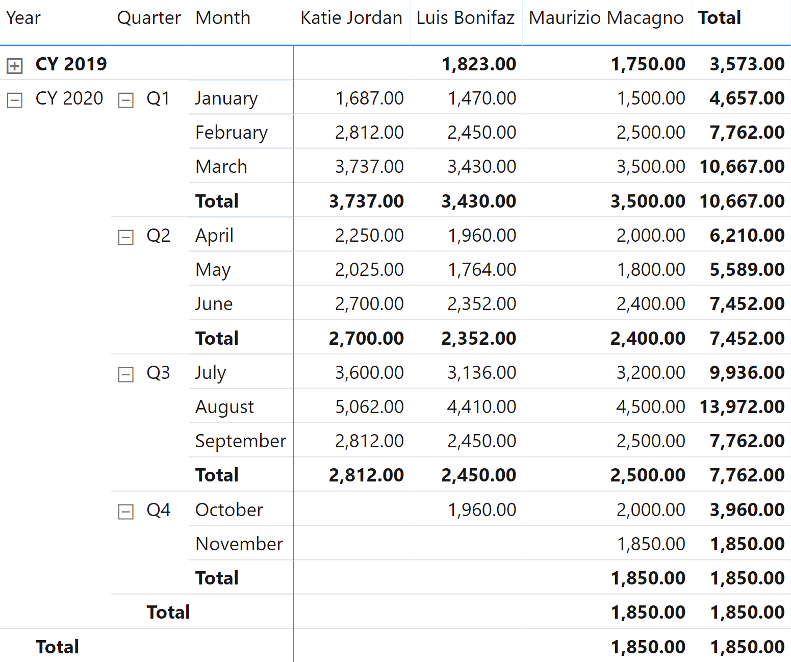
The formula first finds the last date to use, by finding the last date for which there is any data in the model. It then applies it as a filter:

Measure in the Balances table

Balance LastDateWithData :=
VAR MaxBalanceDate =
    CALCULATE (
        MAX ( Balances[Date] ),   -- Use MIN for Balance FirstDateWithData
        ALLEXCEPT (
            Balances,             -- Remove filters from the Balances expanded table
            'Date'                -- but not from the date
        )
    )
VAR Result =
    CALCULATE (
        SUM ( Balances[Balance] ),
        'Date'[Date] = MaxBalanceDate
    )
RETURN
    Result

It is worth noting the presence of ALLEXCEPT in the calculation of MaxBalanceDate. ALLEXCEPT is needed in order to avoid obtaining the last date in the current context, which would use a different date for each customer and at the total level. ALLEXCEPT guarantees that the same date is used for all the customers. In your specific scenario you might have to modify that filter to accommodate for further requirements.

In case you do not want to use the same date for all the customers, but instead you want to use a different date for every customer and total those values, then this is not the right pattern. You need to use the First and last date by customer pattern.

An alternative implementation of this pattern based on LASTNONBLANK is less efficient. It should only be used when the business logic determining whether a date should be considered or not is more complex than just looking at the presence of a row in the Balances table. For example, the following implementation produces the same result as the previous formula with slower execution time and larger memory consumption at query time:

Measure in the Balances table

Slower Balance LastDateWithData :=
CALCULATE (
    SUM ( Balances[Balance] ),
    LASTNONBLANK (
        'Date'[Date],
        CALCULATE ( SUM ( Balances[Balance] ) )
    )
)

First and last date by customer

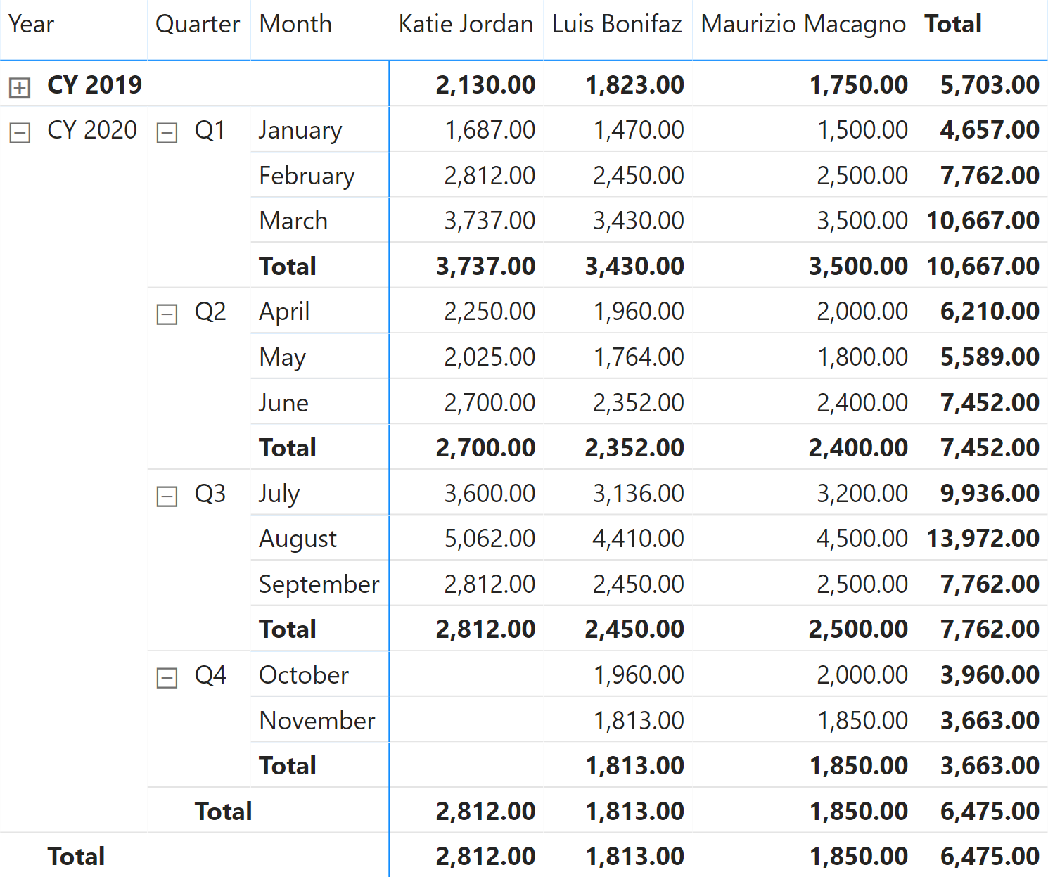
If the dataset contains different dates for each customer – or in general for each entity – then the pattern is different. For each customer you must compute its last date, obtaining the subtotals by summing partial results across other non-date attributes. The result is visible in Figure 4.

The Balance LastDateByCustomer measure provides the desired result:

Measure in the Balances table

Balance LastDateByCustomer :=
VAR MaxBalanceDates =
    ADDCOLUMNS (
        SUMMARIZE (            -- Retrieves the customers
            Balances,          -- from the Balances table
            Customers[Name]
        ),
        "@MaxBalanceDate", CALCULATE (     -- Computes for each customer
            MAX ( Balances[Date] )         -- their last date 
        )
    )
VAR MaxBalanceDatesWithLineage =
    TREATAS (                  -- Changes the lineage of MaxBalanceDates
        MaxBalanceDates,       -- so to make it filter
        Customers[Name],       -- the customer name
        'Date'[Date]           -- and the date
    )
VAR Result =
    CALCULATE (
        SUM ( Balances[Balance] ),
        MaxBalanceDatesWithLineage
    )
RETURN
    Result

In the calculation of the max balance date per customer, you might need to modify the filter further. For example, Katie Jordan reports a blank in Q4 because her last date happens to be outside of the current filter context by quarter. If you need to modify this behavior and report the balance of September forward to the end of the year – and in following years if present – this is achieved by the Balance LastDateByCustomerEver measure:

Measure in the Balances table

Balance LastDateByCustomerEver :=
VAR MaxDate =
    MAX ( 'Date'[Date] )
VAR MaxBalanceDates =
    CALCULATETABLE (
        ADDCOLUMNS (
            SUMMARIZE ( Balances, Customers[Name] ),
            "@MaxBalanceDate", CALCULATE ( MAX ( Balances[Date] ) )
        ),
        'Date'[Date] <= MaxDate
    )
VAR MaxBalanceDatesWithLineage =
    TREATAS ( MaxBalanceDates, Customers[Name], 'Date'[Date] )
VAR Result =
    CALCULATE ( SUM ( Balances[Balance] ), MaxBalanceDatesWithLineage )
RETURN
    Result

You can see the result of the Balance LastDateByCustomerEver measure in Figure 5.

Opening and closing balance

The previous calculations to compute a measure for the last date of a period can be used to compute the closing balance; depending on the requirements, you can choose the right technique. However, the same techniques for the first date cannot be used to retrieve the opening balance, which is usually the closing balance of the previous period.

The Opening measure filters the day before the first day of the period, whereas the Closing measure just gets the last date of the period using LASTDATE:

Measure in the Balances table

Opening := 
VAR PreviousClosingDate =
    DATEADD ( FIRSTDATE ( 'Date'[Date] ), -1, DAY )
VAR Result =
    CALCULATE ( SUM ( Balances[Balance] ), PreviousClosingDate )
RETURN
    Result

Measure in the Balances table

Closing := 
CALCULATE ( 
    SUM ( Balances[Balance] ),
    LASTDATE ( 'Date'[Date] )
)

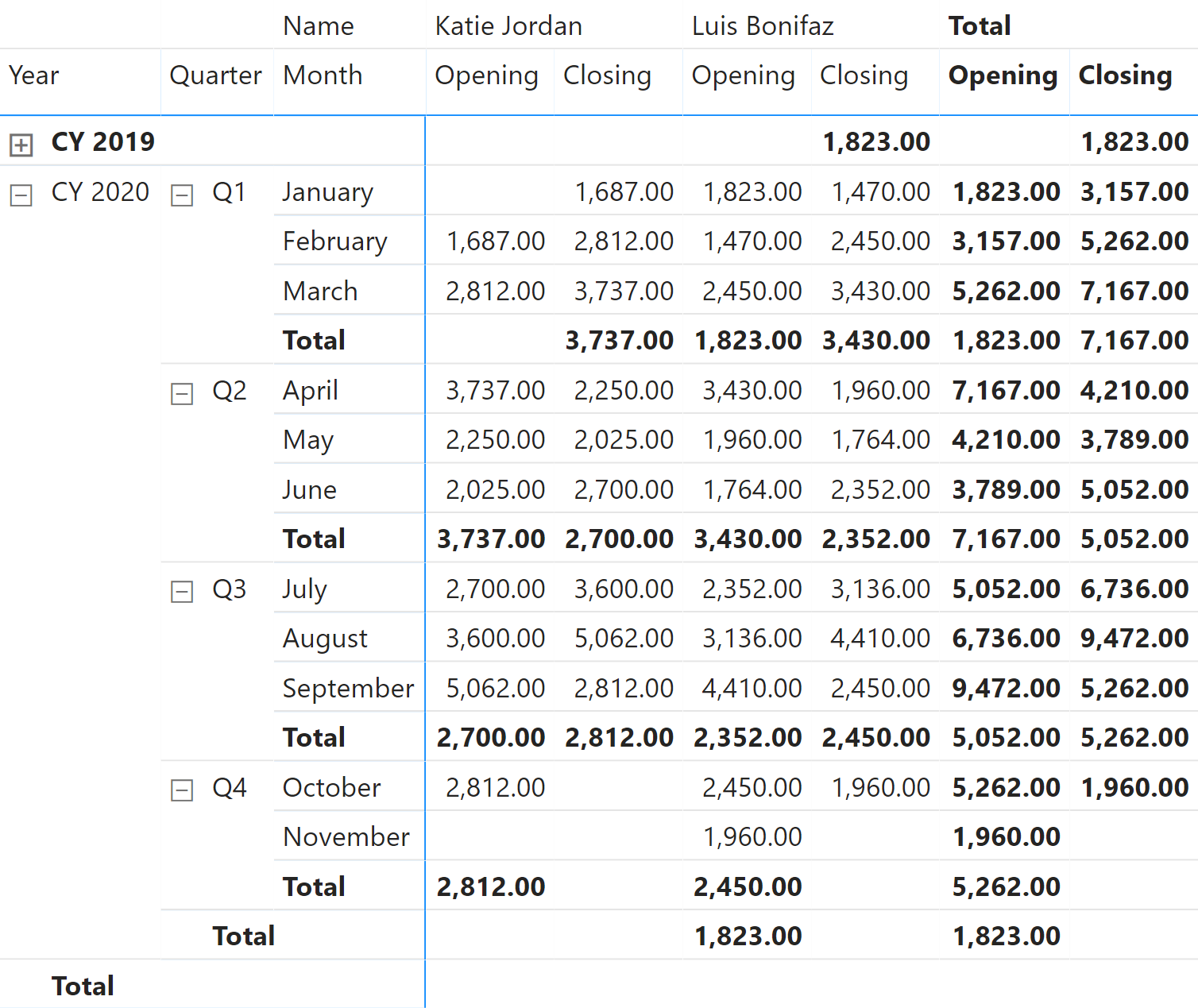
The result in Figure 6 shows that Katie Jordan has an empty opening balance, because the assumption is that the lack of data on December 31, 2019 reflects an empty balance. Indeed, the behavior of the Opening and Closing measures corresponds to the First and last date pattern – which only works if there is a balance for all the customers on the last day of the month.

DAX also provides time intelligence functions for the same purpose, which are specific for each time period considered – month, quarter, or year. However, these functions are slower and they require a more complex DAX syntax in the measures. They should only be considered for measures that always return the opening or closing balance of a specific granularity regardless of the selection. For example, a measure returns the opening or closing balance of the corresponding year, and though the selection might very well be month or quarter the measure would still return the yearly balance.

In our sample report, the CLOSINGBALANCEMONTH can be used instead of CLOSINGBALANCEQUARTER and CLOSINGBALANCEYEAR because they provide the same result for the last month of a period. Similarly, OPENINGBALANCEMONTH can be used instead of OPENINGBALANCEQUARTER and OPENINGBALANCEYEAR because they provide the same result for the first month of a period.

The definition of the Opening Dax and Closing Dax measures is the following:

Measure in the Balances table

Opening Dax :=
OPENINGBALANCEMONTH (
    SUM ( Balances[Balance] ),
    'Date'[Date]
)

Measure in the Balances table

Closing Dax :=
CLOSINGBALANCEMONTH (
    SUM ( Balances[Balance] ),
    'Date'[Date]
)

If you are looking to achieve a behavior matching the First and last date by customer pattern, then you need Balance LastDateByCustomerEver for the implementation of the Closing Ever measure. With a small variation of the same pattern, we are also able to implement the Opening Ever measure:

Measure in the Balances table

Opening Ever :=
VAR MinDate =
    MIN ( 'Date'[Date] )
VAR MaxBalanceDates =
    CALCULATETABLE (
        ADDCOLUMNS (
            SUMMARIZE ( Balances, Customers[Name] ),
            "@MaxBalanceDate", CALCULATE ( MAX ( Balances[Date] ) )
        ),
        'Date'[Date] < MinDate
    )
VAR MaxBalanceDatesWithLineage =
    TREATAS ( MaxBalanceDates, Customers[Name], 'Date'[Date] )
VAR Result =
    CALCULATE ( SUM ( Balances[Balance] ), MaxBalanceDatesWithLineage )
RETURN
    Result

Measure in the Balances table

Closing Ever := 
VAR MaxDate =
    MAX ( 'Date'[Date] )
VAR MaxBalanceDates =
    CALCULATETABLE (
        ADDCOLUMNS (
            SUMMARIZE ( Balances, Customers[Name] ),
            "@MaxBalanceDate", CALCULATE ( MAX ( Balances[Date] ) )
        ),
        'Date'[Date] <= MaxDate
    )
VAR MaxBalanceDatesWithLineage =
    TREATAS ( MaxBalanceDates, Customers[Name], 'Date'[Date] )
VAR Result =
    CALCULATE ( SUM ( Balances[Balance] ), MaxBalanceDatesWithLineage )
RETURN
    Result

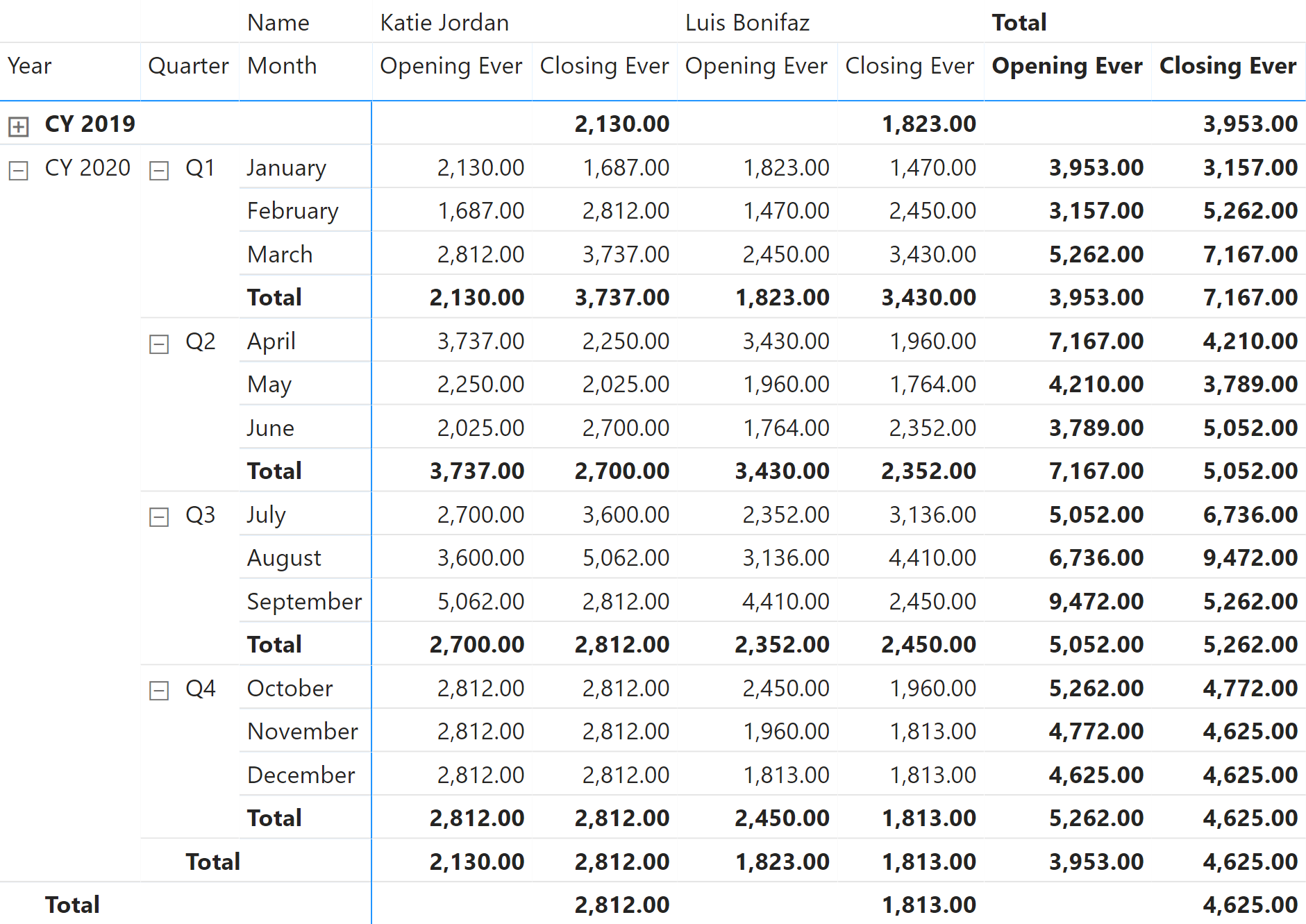
Figure 7 shows that the opening account balance for Katie Jordan for January and Q1 2020 corresponds to the last account balance available in 2019.

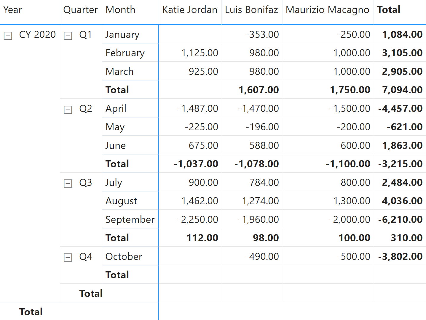
Growth in period

A useful application of this pattern is to compute the variation of a measure over a selected time period. In our example, we want to compute a new measure that produces the difference between the opening and the closing balance for a selected period. The result is visible in Figure 8.

The Growth measure uses the Opening and Closing measures based on the First and last date pattern:

Measure in the Balances table

Growth :=
VAR Opening = [Opening] -- Use Opening Ever if required
VAR Closing = [Closing] -- Use Closing Ever if required
VAR Delta =
    IF ( 
        NOT ISBLANK ( Opening ) && NOT ISBLANK ( Closing ), 
        Closing - Opening 
    )
VAR Result =
    IF ( Delta <> 0, Delta )
RETURN
    Result

As suggested in the comments of the Growth measure, it is possible to use a different logic to obtain the opening and closing balance – by changing the assignment to the Opening and Closing variables. For example, the Growth Ever measure uses the Opening Ever and Closing Ever measures described in the Opening and closing balance pattern:

Measure in the Balances table

Growth Ever :=
VAR Opening = [Opening Ever]
VAR Closing = [Closing Ever]
VAR Delta =
    IF ( 
        NOT ISBLANK ( Opening ) && NOT ISBLANK ( Closing ), 
        Closing - Opening 
    )
VAR Result =
    IF ( Delta <> 0, Delta )
RETURN
    Result

The result of the Growth Ever measure is visible in Figure 9.

Semi-additive calculations

Introduction

First and last date

First and last date with data

First and last date by customer

Opening and closing balance

Growth in period

Video

Downloads

Introduction

First and last date

First and last date with data

First and last date by customer

Opening and closing balance

Growth in period

Video

Do you prefer a video?

Downloads