Custom time-related calculations

This pattern shows how to compute time-related calculations like year-to-date, same period last year, and percentage growth using a custom calendar. This pattern does not rely on DAX built-in time intelligence functions. All the measures refer to the fiscal calendar because the same measures, with a regular Gregorian calendar, can be obtained using the Standard time-related calculations pattern.
UPDATE: There is a new Calendar-based time intelligence feature in Power BI that is in preview from September 2025. We are planning to update the patterns in order to use the new technology, even though we will keep the current article available. While we do not have an exact timeline because the feature is in preview and subject to change, we will certainly publish the updated version of this pattern before the calendar-based time intelligence feature is generally available (GA).
There are several scenarios where the DAX built-in functions for time intelligence cannot provide the right answers. For example, if your fiscal year starts on a month other than January, April, July, or October, then you cannot use the DAX time intelligence functions for quarterly-related calculations. In these scenarios, you need to rewrite the time intelligence logic of the built-in functions by using plain DAX functions like FILTER and CALCULATE. Moreover, you must create a Date table that contains additional columns to compute time periods like the previous quarter or a whole year. Indeed, the standard time intelligence functions derive this information from the Date column in the Date table. The custom time-related calculations pattern does not extract the information from the Date column and requires additional columns.
The measures in this pattern work on a regular Gregorian calendar with the following assumptions:
- Years and quarters always start on the first day of a month.
- A month is always a calendar month.
In simpler words, this pattern works fine if the fiscal year starts on the first day of a month, and a quarter is made of three regular months. For example, if the fiscal year starts on March 3, or all the fiscal quarters must have 90 days, then the formulas do not work.
An example of a calendar that does not satisfy the requirements of this pattern is a week-based calendar. If you need calculations over periods based on weeks, you should use the Week-related calculations pattern.
Introduction to custom time intelligence calculations
The custom time intelligence calculations in this pattern modify the filter context over the Date table to obtain the required result. The formulas are designed to apply filters to the lowest granularity required to improve query performances. For example, a calculation over months works by modifying the filter context at the month level, instead of the individual dates. This technique reduces the cost of computing the new filter and applying it to the filter context. This optimization is especially useful when using DirectQuery, even though it also improves performance on models imported in memory.
Because the pattern does not rely on the standard time intelligence functions, the Date table does not have the requirements needed for standard DAX time intelligence functions.
For example, the Mark as Date Table setting is suggested, but not required. The formulas in this pattern do not rely on the automatic REMOVEFILTERS applied over the Date table when the Date column is filtered. Instead, the Date table must contain specific columns required by the measures. Therefore, although you might already have a Date table in your model, you must read the next section (Building a Date table) to verify that all the required columns are present in the Date table.
Building a Date table
The Date table used for custom time-related calculations is based on the months of the standard Gregorian calendar table. If you already have a Date table, you can import the table and – if necessary – extend it to include a set of columns containing the information required by the DAX formulas. We describe these columns later in this section.
If a Date table is not available, you can create one using a DAX calculated table. As an example, the following DAX expression defines the Date table used in this pattern, which has a fiscal year starting on March 1:
Date =
VAR FirstFiscalMonth = 3  -- First month of the fiscal year
VAR FirstDayOfWeek = 0    -- 0 = Sunday, 1 = Monday, ...
VAR FirstSalesDate = MIN ( Sales[Order Date] )
VAR LastSalesDate = MAX ( Sales[Order Date] )
VAR FirstFiscalYear =     -- Customizes the first fiscal year to use
    YEAR ( FirstSalesDate )
    + 1 * ( MONTH ( FirstSalesDate ) >= FirstFiscalMonth && FirstFiscalMonth > 1)
VAR LastFiscalYear =      -- Customizes the last fiscal year to use
    YEAR ( LastSalesDate )
    + 1 * ( MONTH ( LastSalesDate ) >= FirstFiscalMonth && FirstFiscalMonth > 1)
RETURN
GENERATE (
    VAR FirstDay =
        DATE (
            FirstFiscalYear - 1 * (FirstFiscalMonth > 1),
            FirstFiscalMonth,
            1
        )

    VAR LastDay =
        DATE (
            LastFiscalYear + 1 * (FirstFiscalMonth = 1),
            FirstFiscalMonth, 1
        ) - 1
    RETURN
        CALENDAR ( FirstDay, LastDay ),

    VAR CurrentDate = [Date]
    VAR Yr = YEAR ( CurrentDate )        -- Year Number
    VAR Mn = MONTH ( CurrentDate )       -- Month Number (1-12)
    VAR Mdn = DAY ( CurrentDate )        -- Day of Month
    VAR DateKey = Yr*10000+Mn*100+Mdn
    VAR Wd =                             -- Weekday Number (0 = Sunday, 1 = Monday, ...)
        WEEKDAY ( CurrentDate + 7 - FirstDayOfWeek, 1 )
    VAR WorkingDay =                     -- Working Day (1 = working, 0 = non-working)
        ( WEEKDAY ( CurrentDate, 1 ) IN { 2, 3, 4, 5, 6 } )
    VAR Fyr =                            -- Fiscal Year Number
        Yr + 1 * ( FirstFiscalMonth > 1 && Mn >= FirstFiscalMonth )
    VAR Fmn =                            -- Fiscal Month Number (1-12)
        Mn - FirstFiscalMonth + 1 + 12 * (Mn < FirstFiscalMonth)
    VAR Fqrn =                           -- Fiscal Quarter (string)
        ROUNDUP ( Fmn / 3, 0 )
    VAR Fmqn =
        MOD ( FMn - 1, 3 ) + 1
    VAR Fqr =                            -- Fiscal Quarter (string)
        FORMAT ( Fqrn, "\Q0" )
    VAR FirstDayOfYear =
        DATE ( Fyr - 1 * (FirstFiscalMonth > 1), FirstFiscalMonth, 1 )
    VAR Fydn =
        SUMX (
            CALENDAR ( FirstDayOfYear, CurrentDate ),
            1 * ( MONTH ( [Date] ) <> 2 || DAY ( [Date] ) <> 29 )
        )
    RETURN ROW (
        "DateKey", INT ( DateKey ),
        "Sequential Day Number", INT ( [Date] ),
        "Year Month", FORMAT ( CurrentDate, "mmm yyyy" ),
        "Year Month Number", Yr * 12 + Mn - 1,
        "Fiscal Year", "FY " & Fyr,
        "Fiscal Year Number", Fyr,
        "Fiscal Year Quarter", "F" & Fqr & "-" & Fyr,
        "Fiscal Year Quarter Number", CONVERT ( Fyr * 4 + FQrn - 1, INTEGER ),
        "Fiscal Quarter", "F" & Fqr,
        "Month", FORMAT ( CurrentDate, "mmm" ),
        "Fiscal Month Number", Fmn,
        "Fiscal Month in Quarter Number",  Fmqn,
        "Day of Week", FORMAT ( CurrentDate, "ddd" ),
        "Day of Week Number", Wd,
        "Day of Month Number", Mdn,
        "Day of Fiscal Year Number", Fydn,
        "Working Day", IF ( WorkingDay, "Working Day", "Non-Working Day" )
    )
)
The first two variables are useful to customize the beginning of both the fiscal year and the week. The next variables detect the range of fiscal years required, based on the transactions in Sales. You can customize FirstSalesDate and LastSalesDate to retrieve the first and last transaction date in your model, or you can assign the first and last fiscal year in the FirstFiscalYear and LastFiscalYear variables.
The quarters are computed starting from the first month of the fiscal year. The Date table contains hidden columns to support the correct sorting of years, quarters, and months. These hidden columns are populated with sequential numbers that make it easy to apply filters to retrieve previous or following years, quarters, and months, without relying on complex calculations at query time.
Among the many columns, one is worth expanding on. The Year Month Number column contains the year number multiplied by 12, plus the month. The resulting number is hard to read, but it allows math over months. Given the Year Month Number value, you can just subtract 12 to go back one year; this gives you the value of Year Month Number corresponding to the same month in the previous year. Many formulas use this characteristic to perform time-shifts.
In order to obtain the right visualization, the calendar columns must be configured in the data model as follows – for each column you can see the data type and the format string, followed by a sample value:
- Date: Date, m/dd/yyyy (8/14/2007), used as a column to mark as date table (not required)
- DateKey: Whole Number, (20070814), used as an alternate key for relationships
- Sequential Day Number: Whole Number, Hidden (40040), same value of Date as integer
- Year Month: Text (Aug 2007)
- Year Month Number: Whole Number, Hidden (24091)
- Month: Text (Aug)
- Fiscal Month Number: Whole Number, Hidden (6)
- Fiscal Month in Quarter Number: Whole Number, Hidden (3)
- Fiscal Year: Text (FY 2008)
- Fiscal Year Number: Whole Number, Hidden (2008)
- Fiscal Year Quarter: Text (FQ2-2008)
- Fiscal Year Quarter Number: Whole Number, Hidden (8033)
- Fiscal Quarter: Text (FQ2)
- Day of Fiscal Year Number: Whole Number, Hidden (167)
- Day of Month Number: Whole Number, Hidden (14)
We want to introduce the concept of filter-keep columns. In a table, there are columns whose filters need to be preserved. The filters over filter-keep columns are not altered by the time intelligence calculations. They will be affecting the calculations presented in this pattern. The filter-keep columns in our sample table are the following:
- Day of Week: ddd (Tue)
- Day of Week Number: Whole Number, Hidden (6)
- Working Day: Text (Working Day)
We further describe the behavior of filter-keep columns in the next section.
The Date table in this pattern has one hierarchy:
- Fiscal: Year (Fiscal Year), Quarter (Fiscal Year Quarter), Month (Year Month)
The columns are designed to simplify the formulas. For example, the Day of Fiscal Year Number column contains the number of days since the beginning of the fiscal year, ignoring February 29 in leap years; this number makes it easier to find a corresponding range of dates in the previous year.
The Date table must also include a hidden DateWithSales calculated column, used by some of the formulas of this pattern:
DateWithSales =
'Date'[Date] <= MAX ( Sales[Order Date] )
The Date[DateWithSales] column is TRUE if the date is on or before the last date with sales; it is FALSE otherwise. In other words, DateWithSales is TRUE for “past” dates and FALSE for “future” dates, where “past” and “future” are relative to the last date with sales.
In case you import a Date table, you want to create columns that are similar to the ones we describe in this pattern, in that they should behave the same way.
Understanding filter-keep columns
The Date table contains two types of columns: regular columns and filter-keep columns. The regular columns are manipulated by the measures shown in this pattern. The filters over filter-keep columns are always preserved and never altered by the measures of this pattern. An example clarifies this distinction. The Year Month Number column is a regular column: the formulas in this pattern have the option of changing its value during their computation.
For example, in order to compute the previous month the formulas change the filter context by subtracting one to the value of Year Month Number in the filter context. Conversely, the Day of Week column is a filter-keep column. If a user filters Monday to Friday, the formulas do not alter that filter on the day of the week. Therefore, a previous-year measure keeps the filter on the day of the week; it replaces only the filter on calendar columns such as year, month, and date.
To implement this pattern, you must identify which columns need to be treated as filter-keep columns, because filter-keep columns require special handling. The following is the classification of the columns used in the Date table of this pattern:
- Calendar columns: Date, DateKey, Sequential Day Number, Year Month, Year Month Number, Month, Fiscal Month Number, Fiscal Month in Quarter Number, Fiscal Year, Fiscal Year Number, Fiscal Year Quarter, Fiscal Year Quarter Number, Fiscal Quarter, Day of Fiscal Year Number, Day of Month Number .
- Filter-keep columns: Day of Week, Day of Week Number, Working Day.
The special handling of filter-keep columns pertains to the filter context. Every measure in this pattern manipulates the filter context by replacing filters over all the calendar columns, without altering any filter applied to the filter-keep columns. In other words, every measure follows two rules:
- Remove filters on calendar columns;
- Keep filters on filter-keep columns.
The ALLEXCEPT function can implement these requirements; specify the Date table in the first argument, and the filter-keep columns in the following arguments:
CALCULATE (
    [Sales Amount],
    ALLEXCEPT ( 'Date', 'Date'[Working Day], 'Date'[Day of Week] ),
    ... // Filters over one or more calendar columns
)
If the Date table did not have any filter-keep column, the filters could be removed by using REMOVEFILTERS over the Date table instead of ALLEXCEPT:
CALCULATE (
    [Sales Amount],
    REMOVEFILTERS ( 'Date' ),
    ... // Filters over one or more calendar columns
)
If your Date table does not contain any filter-keep column, then you can use REMOVEFILTERS instead of ALLEXCEPT in all the measures of this pattern. We provide a complete scenario that includes filter-keep columns. Whenever possible, you can simplify it.
While the ALLEXCEPT should include all the filter-keep columns, we skip specifically the hidden filter-keep columns used only to sort other columns. For example, we do not include Day of Week Number, which is a hidden column used to sort the Day of Week column. The assumption is that the user never applies filters on hidden columns; if this assumption is not true, then the hidden filter-keep columns must also be included in the ALLEXCEPT arguments. You can find an example of the different results of using REMOVEFILTERS and ALLEXCEPT in the Year-to-date total section of this pattern.
Controlling the visualization on future dates
Most of the time intelligence calculations should not display values for dates after the last date available. For example, a year-to-date calculation can also show values for future dates, but we want to hide those values. The dataset used in these examples ends on August 15, 2009. Therefore, we consider the month of August 2009, the third quarter of 2009 (Q3-2009), and the year 2009 as the last time periods with data. Any date later than August 15, 2019 is considered future, and we want to hide its values.
In order to avoid showing results in future dates, we use the following ShowValueForDates measure. ShowValueForDates returns TRUE if the period selected is earlier than the last period with data:
ShowValueForDates :=
VAR LastDateWithData =
    CALCULATE (
        MAX ( 'Sales'[Order Date] ),
        REMOVEFILTERS ()
    )
VAR FirstDateVisible =
    MIN ( 'Date'[Date] )
VAR Result =
    FirstDateVisible <= LastDateWithData
RETURN
    Result
The ShowValueForDates measure is hidden. It is a technical measure created to reuse the same logic in many different time-related calculations, and the user should not use ShowValueForDates directly in a report. The REMOVEFILTERS function removes filters from all tables in the model, because the purpose is to retrieve the last date used in the Sales table regardless of filters.
Naming convention
This section describes the naming convention we adopted to reference the time intelligence calculations. A simple categorization shows whether a calculation:
- Shifts over a period of time, for example the same period in the previous year;
- Performs an aggregation, for example year-to-date; or,
- Compares two time periods, for example this year compared to last year.
| Acronym | Description | Shift | Aggregation | Comparison |
| YTD | Year-to-date | |||
| QTD | Quarter-to-date | |||
| MTD | Month-to-date | |||
| MAT | Moving annual total | |||
| PY | Previous year | |||
| PQ | Previous quarter | |||
| PM | Previous month | |||
| PYC | Previous year complete | |||
| PQC | Previous quarter complete | |||
| PMC | Previous month complete | |||
| PP | Previous period (automatically selects year, quarter, or month) | |||
| PYMAT | Previous year moving annual total | |||
| YOY | Year-over-year | |||
| QOQ | Quarter-over-quarter | |||
| MOM | Month-over-month | |||
| MATG | Moving annual total growth | |||
| POP | Period-over-period (automatically selects year, quarter, or month) | |||
| PYTD | Previous year-to-date | |||
| PQTD | Previous quarter-to-date | |||
| PMTD | Previous month-to-date | |||
| YOYTD | Year-over-year-to-date | |||
| QOQTD | Quarter-over-quarter-to-date | |||
| MOMTD | Month-over-month-to-date | |||
| YTDOPY | Year-to-date-over-previous-year | |||
| QTDOPQ | Quarter-to-date-over-previous-quarter | |||
| MTDOPM | Month-to-date-over-previous-month |
Computing period-to-date totals
The year-to-date, quarter-to-date, and month-to-date calculations modify the filter context for the Date table, showing the values from the beginning of the period up to the last date available in the filter context.
Year-to-date total
The year-to-date aggregates data starting from the first day of the fiscal year, as shown in Figure 1.
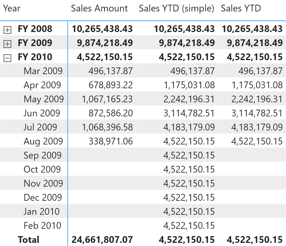
The measure filters all the days less than or equal to the last day visible in the last fiscal year. It also filters the last visible Fiscal Year Number:
Sales YTD (simple) :=
VAR LastDayAvailable = MAX ( 'Date'[Day of Fiscal Year Number] )
VAR LastFiscalYearAvailable = MAX ( 'Date'[Fiscal Year Number] )
VAR Result =
    CALCULATE (
        [Sales Amount],
        ALLEXCEPT ( 'Date', 'Date'[Working Day], 'Date'[Day of Week] ),
        'Date'[Day of Fiscal Year Number] <= LastDayAvailable,
        'Date'[Fiscal Year Number] = LastFiscalYearAvailable
    )
RETURN
    Result
Because LastDayAvailable contains the last date visible in the filter context, Sales YTD (simple) shows data even for future dates in the year. We can prevent this behavior in the Sales YTD measure by returning a result only when ShowValueForDates returns TRUE:
Sales YTD :=
IF (
    [ShowValueForDates],
    VAR LastDayAvailable =  MAX ( 'Date'[Day of Fiscal Year Number] )
    VAR LastFiscalYearAvailable = MAX ( 'Date'[Fiscal Year Number] )
    VAR Result =
        CALCULATE (
            [Sales Amount],
            ALLEXCEPT ( 'Date', 'Date'[Working Day], 'Date'[Day of Week] ),
            'Date'[Day of Fiscal Year Number] <= LastDayAvailable,
            'Date'[Fiscal Year Number] = LastFiscalYearAvailable
        )
    RETURN
        Result
)
ALLEXCEPT is required to preserve the filter-keep columns Working Day or Day of Week in case they are used in the report. To demonstrate this, we created an incorrect measure: Sales YTD (wrong), which removes the filters from the Date table by using REMOVEFILTERS instead of ALLEXCEPT. By doing this, the formula loses the filter on Working Day used in the columns of the matrix, thus returning an inaccurate result:
Sales YTD (wrong) :=
IF (
    [ShowValueForDates],
    VAR LastDayAvailable =  MAX ( 'Date'[Day of Fiscal Year Number] )
    VAR LastFiscalYearAvailable = MAX ( 'Date'[Fiscal Year Number] )
    VAR Result =
        CALCULATE (
            [Sales Amount],
            REMOVEFILTERS ( 'Date' ),
            'Date'[Day of Fiscal Year Number] <= LastDayAvailable,
            'Date'[Fiscal Year Number] = LastFiscalYearAvailable
        )
    RETURN
        Result
)
Figure 2 shows the comparison of the correct and incorrect measures.
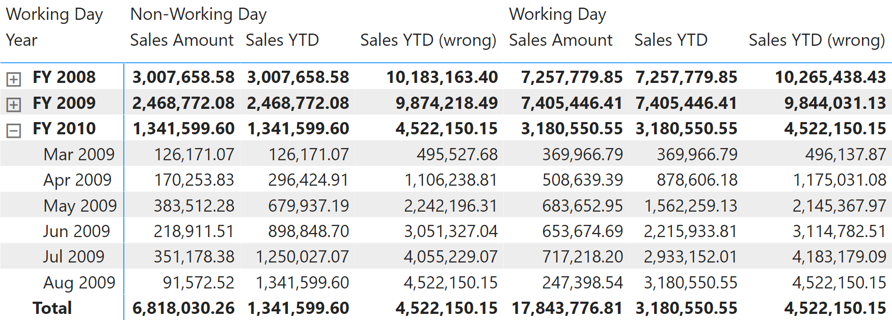
The Sales YTD (wrong) measure would work well if the Date table did not contain any filter-keep columns. The presence of filter-keep columns requires the use of ALLEXCEPT instead of REMOVEFILTERS. We used Sales YTD as an example, but the same concept is valid for all the other measures in this pattern.
Quarter-to-date total
Quarter-to-date aggregates data starting from the first day of the fiscal quarter, as shown in Figure 3.
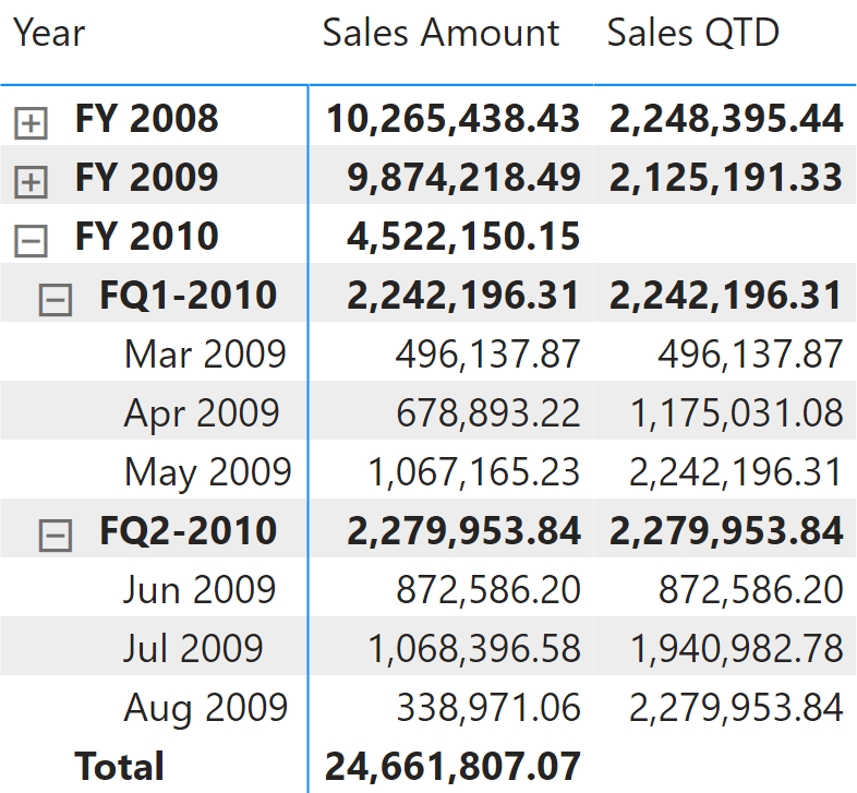
The quarter-to-date value is computed using the same technique as the one used for the year-to-date total. The only difference is the filter on Fiscal Year Quarter Number instead of on Fiscal Year Number:
Sales QTD :=
IF (
    [ShowValueForDates],
    VAR LastDayAvailable = MAX ( 'Date'[Day of Fiscal Year Number] )
    VAR LastFiscalYearQuarterAvailable = MAX ( 'Date'[Fiscal Year Quarter Number] )
    VAR Result =
        CALCULATE (
            [Sales Amount],
            ALLEXCEPT ( 'Date', 'Date'[Working Day], 'Date'[Day of Week] ),
            'Date'[Day of Fiscal Year Number] <= LastDayAvailable,
            'Date'[Fiscal Year Quarter Number] = LastFiscalYearQuarterAvailable
        )
    RETURN
        Result
)
Month-to-date total
The month-to-date aggregates data from the first day of the month, as shown in Figure 4.
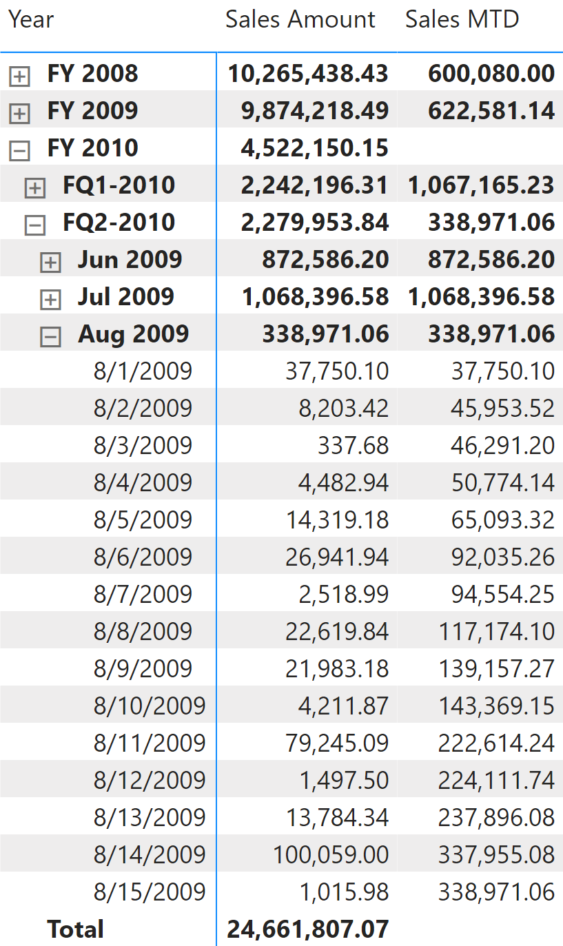
The month-to-date total is computed with a technique similar to the technique used in year-to-date total and quarter-to-date total. It filters all the days that are less than or equal to the last day visible in the last month. The filters are applied to the Day of Month Number and Year Month Number columns:
Sales MTD :=
IF (
    [ShowValueForDates],
    VAR LastDayAvailable =  MAX ( 'Date'[Day of Month Number] )
    VAR LastFiscalYearMonthAvailable = MAX ( 'Date'[Year Month Number] )
    VAR Result =
        CALCULATE (
            [Sales Amount],
            ALLEXCEPT ( 'Date', 'Date'[Working Day], 'Date'[Day of Week] ),
            'Date'[Day of Month Number] <= LastDayAvailable,
            'Date'[Year Month Number] = LastFiscalYearMonthAvailable
        )
    RETURN
        Result
)
The measure filters Day of Month Number instead of Day of Fiscal Year Number. The goal is to filter a column with a lower number of unique values, which is a best practice from a query performance standpoint (the quarter-to-date total does not apply this optimization because the performance advantage would be minimal).
Computing period-over-period growth
A common requirement is to compare a time period with the same period in the previous year, quarter, or month. The last month/quarter/year could be incomplete. In order to achieve a fair comparison, the measure should work on an equivalent time period. For these reasons, the calculations shown in this section use the Date[DateWithSales] calculated column as described in the article, Hiding future dates for calculations in DAX.
Year-over-year growth
Year-over-year compares a time period to its equivalent in the previous year. In this example, data is available until August 15, 2009. For this reason, Sales PY shows numbers related to FY 2010, and just considers transactions made before August 15, 2008. Figure 5 shows that Sales Amount in August 2009 is 721,560.95, whereas Sales PY in August 2009 returns 296,529.51 because the measure considers only the sales made up to August 15, 2008.
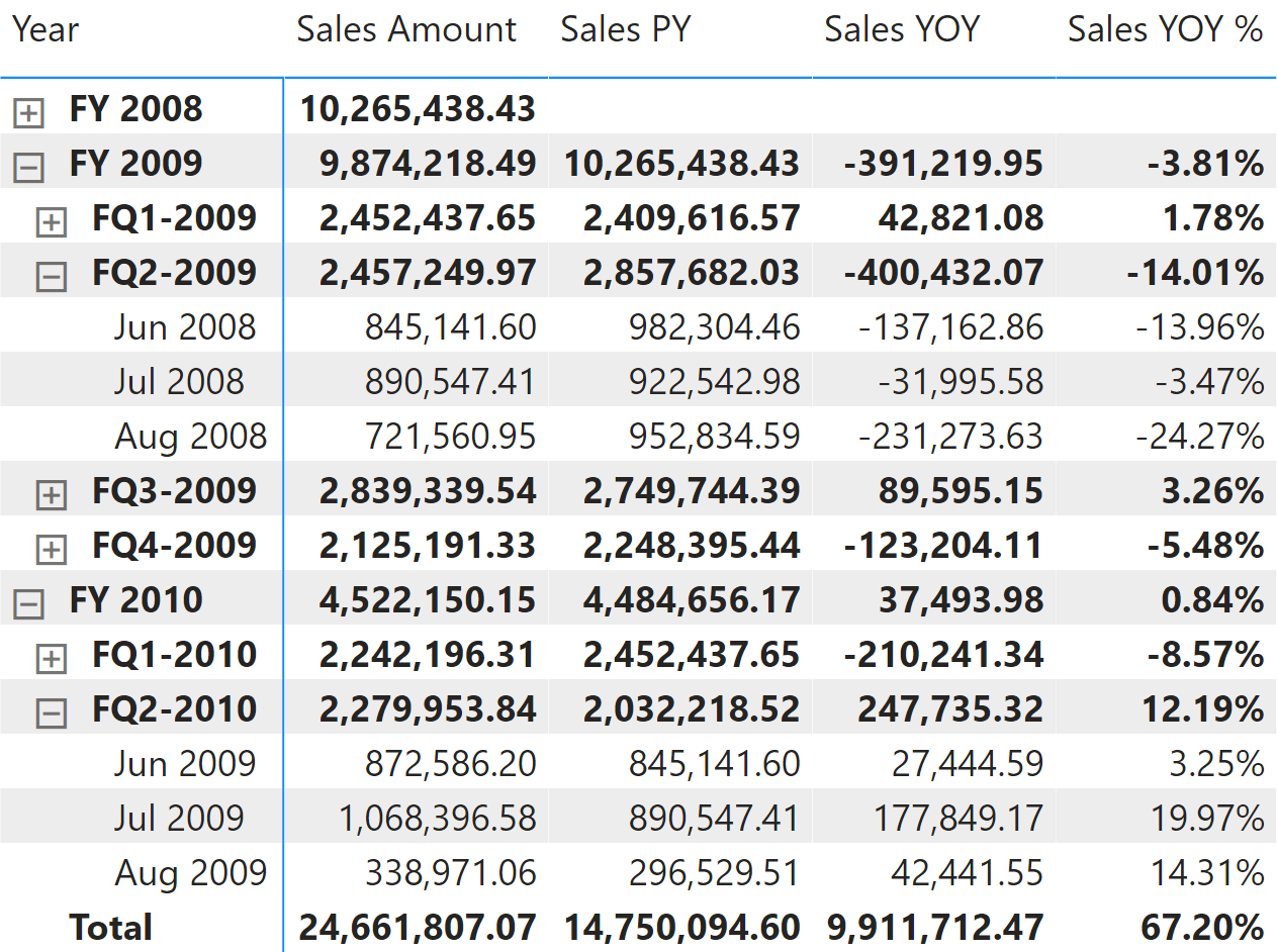
Sales PY uses a standard technique that shifts the selection by the number of months defined in the MonthsOffset variable. In Sales PY the variable is set to 12, to move time back by 12 months. The next measures Sales PQ and Sales PM use the same code, the only difference being the value assigned to MonthsOffset.
Sales PY iterates every month active in the filter context. For each month, it checks whether the days selected in the month correspond to all the days of the month, taking into account the filter-keep columns – Working Day and Day of Week in our example. If all the days are selected, it means that the current filter context includes a full month. Therefore, the filter is shifted back to the previous full month. If not all the days are selected, it means that the user has placed one or more filters on calendar columns that show a partial month. In that case, the selected days are shifted back in the corresponding month of the previous year. The filter over Date[DateWithSales] guarantees a fair comparison with the last period with data:
Sales PY :=
VAR MonthsOffset = 12
RETURN IF (
    [ShowValueForDates],
    SUMX (
        SUMMARIZE ( 'Date', 'Date'[Year Month Number] ),
        VAR CurrentYearMonthNumber = 'Date'[Year Month Number]
        VAR PreviousYearMonthNumber = CurrentYearMonthNumber - MonthsOffset
        VAR DaysOnMonth =
            CALCULATE (
                COUNTROWS ( 'Date' ),
                ALLEXCEPT (
                    'Date',
                    'Date'[Year Month Number],  -- Year Month granularity
                    'Date'[Working Day],        -- Filter-keep Date column
                    'Date'[Day of week]         -- Filter-keep Date column
                )
            )
        VAR DaysSelected =
            CALCULATE (
                COUNTROWS ( 'Date' ),
                'Date'[DateWithSales] = TRUE
            )
        RETURN IF (
            DaysOnMonth = DaysSelected,

            -- Selection of all days in the month
            CALCULATE (
                [Sales Amount],
                ALLEXCEPT ( 'Date', 'Date'[Working Day], 'Date'[Day of Week] ),
                'Date'[Year Month Number] = PreviousYearMonthNumber
            ),

            -- Partial selection of days in a month
            CALCULATE (
                [Sales Amount],
                ALLEXCEPT ( 'Date', 'Date'[Working Day], 'Date'[Day of Week] ),
                'Date'[Year Month Number] = PreviousYearMonthNumber,
                CALCULATETABLE (
                    VALUES ( 'Date'[Day of Month Number] ),
                    ALLEXCEPT (                      -- Removes filters from all the
                        'Date',                      -- columns that do not have a day
                        'Date'[Day of Month Number], -- granularity, keeping only
                        'Date'[Date]                 -- Date and Day of Month Number
                    ),
                    'Date'[Year Month Number] = CurrentYearMonthNumber,
                    'Date'[DateWithSales] = TRUE
                )
            )
        )
    )
)
The year-over-year growth is computed as an amount in Sales YOY, and as a percentage in Sales YOY %. Both measures use Sales PY to consider only dates up to August 15, 2009:
Sales YOY :=
VAR ValueCurrentPeriod = [Sales Amount]
VAR ValuePreviousPeriod = [Sales PY]
VAR Result =
    IF (
        NOT ISBLANK ( ValueCurrentPeriod )
            && NOT ISBLANK ( ValuePreviousPeriod ),
        ValueCurrentPeriod - ValuePreviousPeriod
    )
RETURN
    Result
Sales YOY % :=
DIVIDE (
    [Sales YOY],
    [Sales PY]
)
Quarter-over-quarter growth
Quarter-over-quarter compares a time period with its equivalent in the previous quarter. In this example, data is available until August 15, 2009, which is the first 15 days of the third month in the second quarter of FY 2010. Therefore, Sales PQ for August 2009 (the third month of the second quarter) shows sales until May 15, 2009, which is the first 15 days of the third month of the previous quarter. Figure 6 shows that Sales Amount in May 2009 is 1,067,165.23, whereas Sales PQ in August 2009 returns 435,306.10 thus only taking into account sales made up to May 15, 2009.
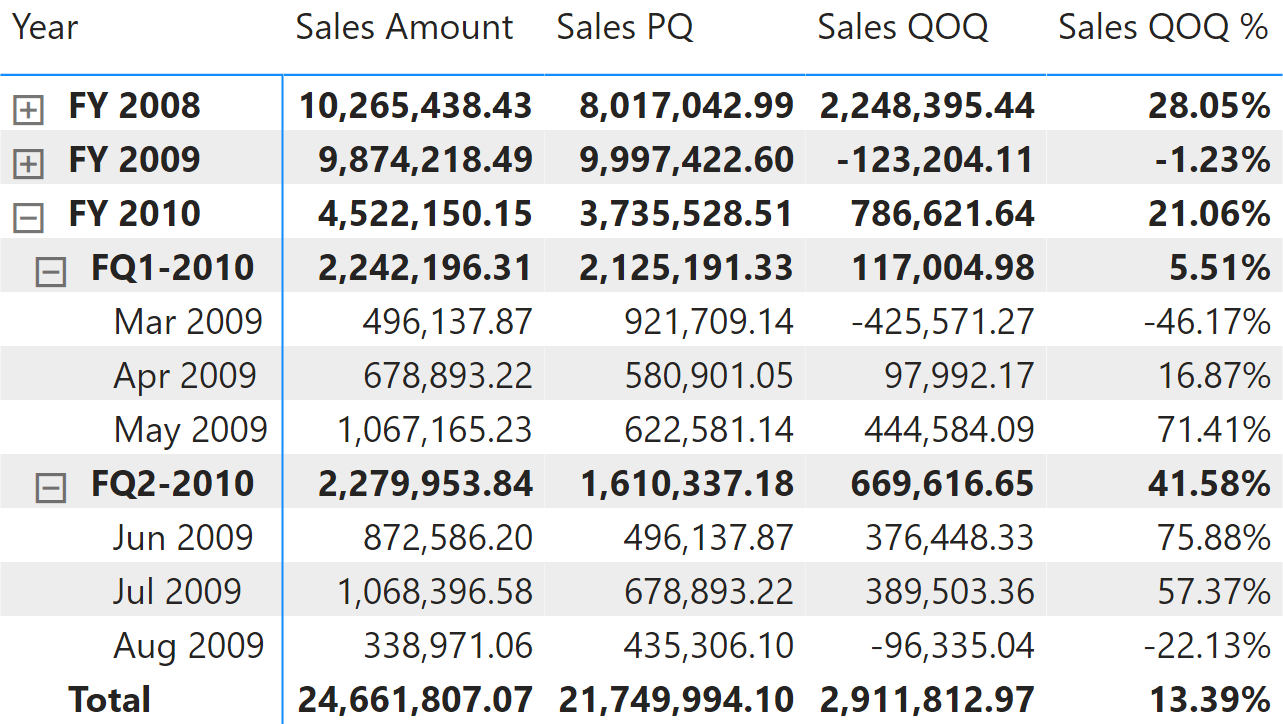
Sales PQ also uses the technique described for Sales PY. The only difference is that MonthsOffset is set to 3 months instead of 12:
Sales PQ :=
VAR MonthsOffset = 3
... // Same definition as Sales PY
The quarter-over-quarter growth is computed as an amount in Sales QOQ and as a percentage in Sales QOQ %. Both measures use Sales PQ to guarantee a fair comparison:
Sales QOQ :=
VAR ValueCurrentPeriod = [Sales Amount]
VAR ValuePreviousPeriod = [Sales PQ]
VAR Result =
    IF (
        NOT ISBLANK ( ValueCurrentPeriod )
            && NOT ISBLANK ( ValuePreviousPeriod ),
        ValueCurrentPeriod - ValuePreviousPeriod
    )
RETURN
    Result
Sales QOQ % :=
DIVIDE (
    [Sales QOQ],
    [Sales PQ]
)
Month-over-month growth
Month-over-month compares a time period with its equivalent in the previous month. In this example, data is only available until August 15, 2009. For this reason, Sales PM only takes sales between July 1-15, 2009 into account in order to return a value for August 2009. That way, it only returns the corresponding portion of the previous month. Figure 7 shows that Sales Amount for July 2009 is 1,068,396.58, whereas Sales PM of August 2019 returns 584,212.78 – since it only takes into account sales up to July 15, 2009.
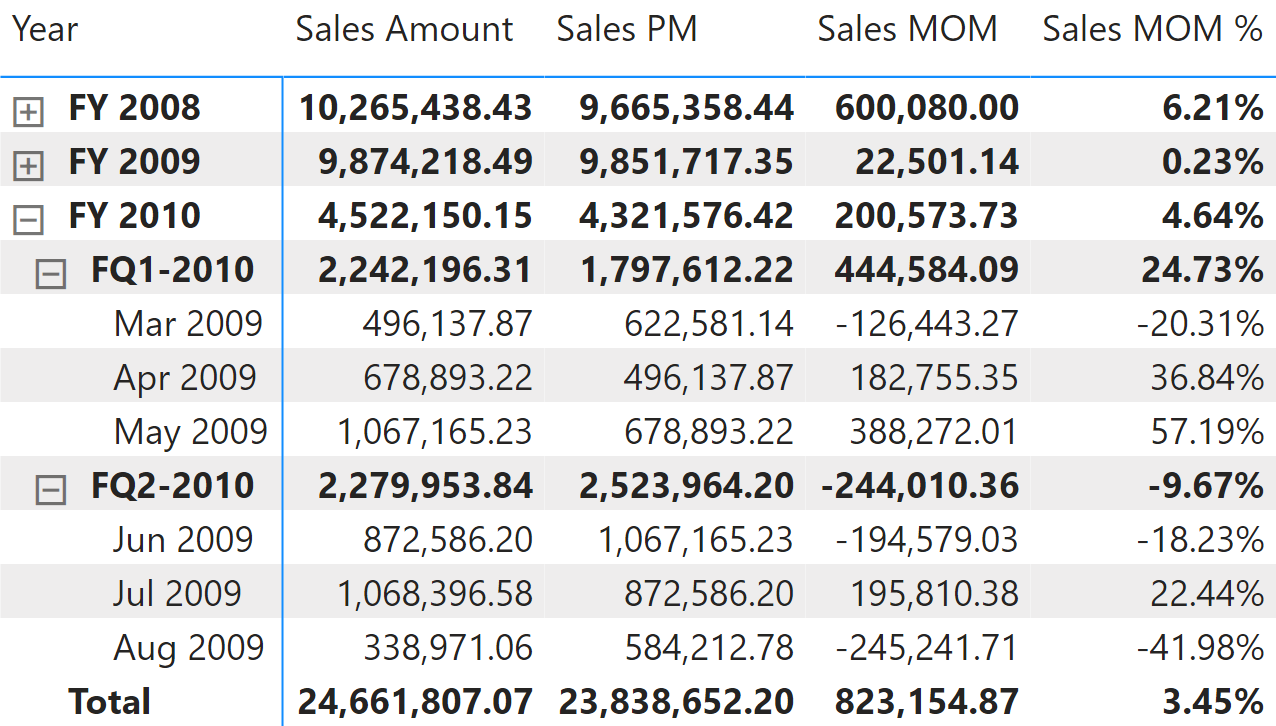
Sales PM uses the technique described for Sales PY. The only difference is that MonthsOffset is set to 1 month instead of 12:
Sales PM :=
VAR MonthsOffset = 1
... // Same definition as Sales PY
The month-over-month growth is computed as an amount in Sales MOM and as a percentage in Sales MOM %. Both measures use Sales PM to guarantee a fair comparison:
Sales MOM :=
VAR ValueCurrentPeriod = [Sales Amount]
VAR ValuePreviousPeriod = [Sales PM]
VAR Result =
    IF (
        NOT ISBLANK ( ValueCurrentPeriod )
            && NOT ISBLANK ( ValuePreviousPeriod ),
        ValueCurrentPeriod - ValuePreviousPeriod
    )
RETURN
    Result
Sales MOM % :=
DIVIDE (
    [Sales MOM],
    [Sales PM]
)
Period-over-period growth
Period-over-period growth automatically selects one of the measures previously described in this section based on the current selection of the visualization. For example, it returns the value of month-over-month growth measures if the visualization displays data at the month level; but it switches to year-over-year growth measures if the visualization shows the total at the year level. The result is visible in Figure 8.
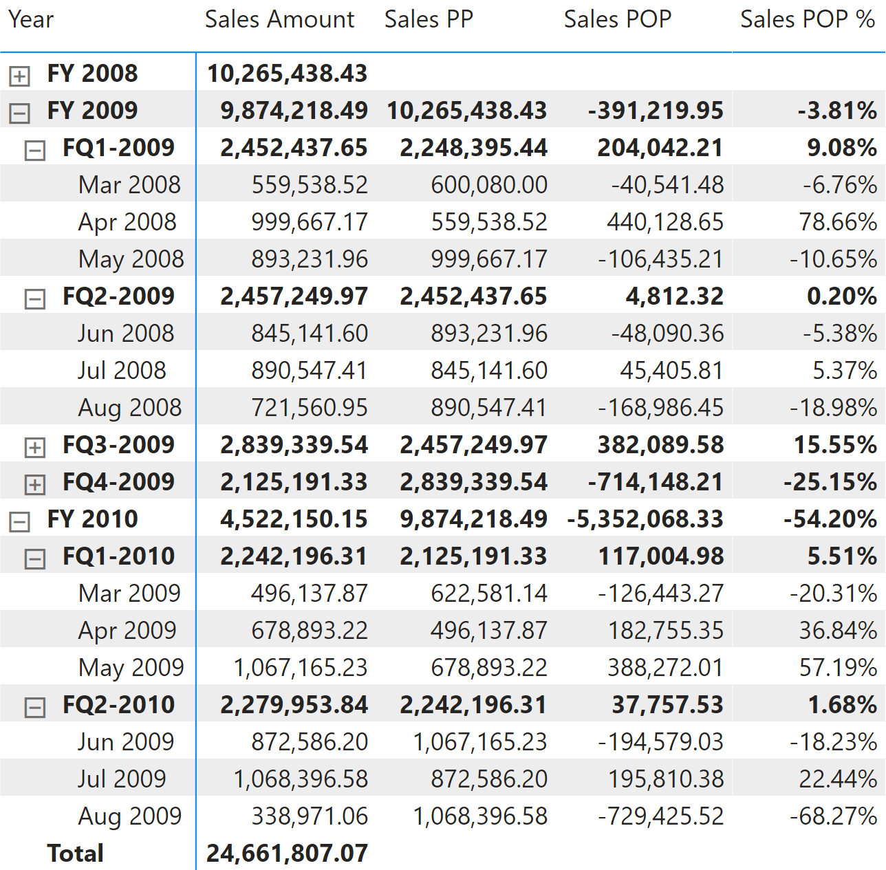
The three measures Sales PP, Sales POP, and Sales POP % redirect the evaluation to the corresponding year, quarter, and month measures depending on the level selected in the report. ISINSCOPE detects the level used in the report. The arguments passed to ISINSCOPE are the attributes used in the rows of the Matrix visual in Figure 8. The measures are defined as follows:
Sales POP % :=
SWITCH (
    TRUE,
    ISINSCOPE ( 'Date'[Year Month] ), [Sales MOM %],
    ISINSCOPE ( 'Date'[Fiscal Year Quarter] ), [Sales QOQ %],
    ISINSCOPE ( 'Date'[Fiscal Year] ), [Sales YOY %]
)
Sales POP :=
SWITCH (
    TRUE,
    ISINSCOPE ( 'Date'[Year Month] ), [Sales MOM],
    ISINSCOPE ( 'Date'[Fiscal Year Quarter] ), [Sales QOQ],
    ISINSCOPE ( 'Date'[Fiscal Year] ), [Sales YOY]
)
Sales PP :=
SWITCH (
    TRUE,
    ISINSCOPE ( 'Date'[Year Month] ), [Sales PM],
    ISINSCOPE ( 'Date'[Fiscal Year Quarter] ), [Sales PQ],
    ISINSCOPE ( 'Date'[Fiscal Year] ), [Sales PY]
)
Computing period-to-date growth
The growth of a “to-date” measure is the comparison of the “to-date” measure with the same measure over an equivalent period with a specific offset. For example, you can compare a year-to-date aggregation against the year-to-date in the previous year, that is with an offset of one year.
All the measures in this set of calculations take care of partial time periods. Because data is available only until August 15, 2009 in our example, the measures make sure the previous year does not report dates after August 15, 2008.
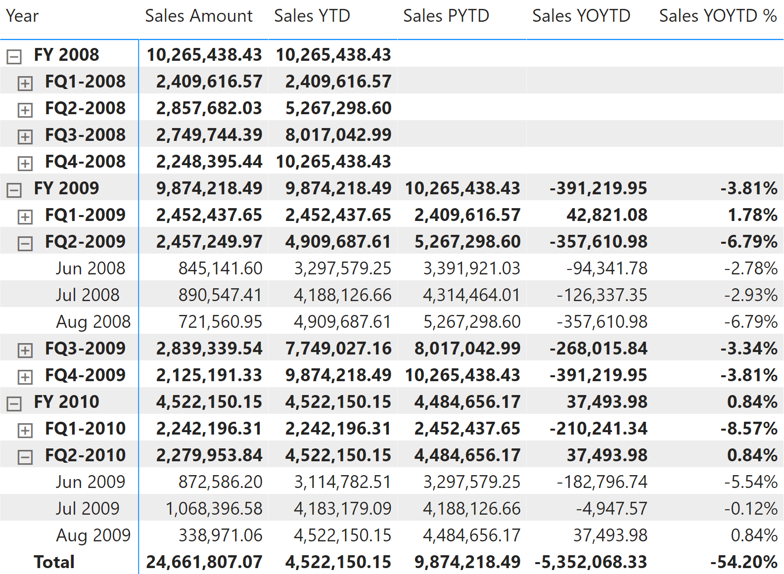
Year-over-year-to-date growth
Year-over-year-to-date growth compares the year-to-date at a specific date with the year-to-date at an equivalent date in the previous year. Figure 9 shows that Sales PYTD in FY 2010 is considering only sales until August 15, 2008. For this reason, Sales YTD of FQ2-2009 is 4,909,687.61, whereas Sales PYTD for FQ2-2010 is less at 4,484,656.17.
Sales PYTD is like Sales YTD, in that it filters the previous value in Fiscal Year Number instead of the last year visible in the filter context. The main difference is the evaluation of LastDayOfFiscalYearAvailable; it must take into account only dates with sales, and ignore the filter on filter-keep columns which matter in the evaluation of Sales Amount:
Sales PYTD :=
IF (
    [ShowValueForDates],
    VAR PreviousFiscalYear = MAX ( 'Date'[Fiscal Year Number] ) - 1
    VAR LastDayOfFiscalYearAvailable =
        CALCULATE (
            MAX ( 'Date'[Day of Fiscal Year Number] ),
            REMOVEFILTERS (                -- Removes filters from
                'Date'[Working Day],       -- filter-keep columns
                'Date'[Day of Week],       -- to get the last day with data
                'Date'[Day of Week Number] -- selected in the report
            ),
            'Date'[DateWithSales] = TRUE
        )
    VAR Result =
        CALCULATE (
            [Sales Amount],
            ALLEXCEPT ( 'Date', 'Date'[Working Day], 'Date'[Day of Week] ),
            'Date'[Fiscal Year Number] = PreviousFiscalYear,
            'Date'[Day of Fiscal Year Number] <= LastDayOfFiscalYearAvailable,
            'Date'[DateWithSales] = TRUE
        )
    RETURN
        Result
)
Sales YOYTD and Sales YOYTD % rely on Sales PYTD to guarantee a fair comparison:
Sales YOYTD :=
VAR ValueCurrentPeriod = [Sales YTD]
VAR ValuePreviousPeriod = [Sales PYTD]
VAR Result =
    IF (
        NOT ISBLANK ( ValueCurrentPeriod ) && NOT ISBLANK ( ValuePreviousPeriod ),
        ValueCurrentPeriod - ValuePreviousPeriod
    )
RETURN
    Result
Sales YOYTD % :=
DIVIDE (
    [Sales YOYTD],
    [Sales PYTD]
)
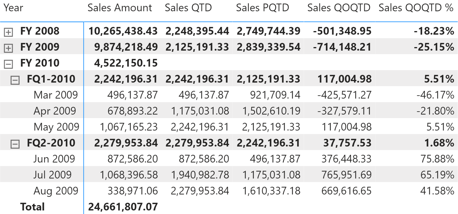
Quarter-over-quarter-to-date growth
Quarter-over-quarter-to-date growth compares the quarter-to-date at a specific date with the quarter-to-date at an equivalent date in the previous quarter. Figure 10 shows that Sales PQ in August 2009 is just taking into account transactions performed up to May 15, 2009, to get the corresponding part of the previous quarter. For this reason Sales QTD of May 2009 is 2,242,196.31, whereas Sales PQTD for August 2009 is lower at 1,610,337.18.
Sales PQTD performs several steps, some of which are somewhat complex. The first two variables are quite easy: LastMonthSelected contains the last month visible in the filter context, while DaysOnLastMonth contains the number of days in LastMonthSelected.
It is important to note that if DaysOnLastMonth is equal to DaysLastMonthSelected, it means that the current filter context includes the end of a month; therefore the corresponding selection in the previous quarter must include the entire relative month. If DaysOnLastMonth is not equal to DaysLastMonthSelected, then the filter context is restricting the number of visible days. Consequently, we compute the last day of the month with data and we restrict the result to go only up to the same day number in the relative month within the previous quarter. This calculation takes place in LastDayOfMonthWithSales, which contains the last day of the month with sales regardless of the filter-keep columns.
If the selection in the last month includes the whole month, then LastDayOfMonthWithSales contains the fixed value 31, which is a number greater than or equal to all the other days of a month. A similar calculation occurs with LastMonthInQuarterWithSales, this time with the month number. These two variables are used to compute FilterQTD in the last step. FilterQTD contains all the pairs of (FiscalMonthInQuarter, FiscalDayInMonth) that are less than or equal to the pair (LastMonthInQuarterWithSales, LastDayOfMonthWithSales). By using ISONORAFTER ( …, DESC ) we obtain the effect we would get by using NOT ISONORAFTER with the default ASC sort order:
Sales PQTD :=
IF (
    [ShowValueForDates],
    VAR LastMonthSelected =
        MAX ( 'Date'[Year Month Number] )
    VAR DaysOnLastMonth =
        CALCULATE (
            COUNTROWS ( 'Date' ),
            ALLEXCEPT ( 'Date', 'Date'[Working Day], 'Date'[Day of week] ),
            'Date'[Year Month Number] = LastMonthSelected
        )
    VAR DaysLastMonthSelected =
        CALCULATE (
            COUNTROWS ( 'Date' ),
            'Date'[DateWithSales] = TRUE,
            'Date'[Year Month Number] = LastMonthSelected
        )
    VAR LastDayOfMonthWithSales =
        MAX (
            -- End of month of any month
            31 * (DaysOnLastMonth = DaysLastMonthSelected),
            -- or last day selected with data
            CALCULATE (
                MAX ( 'Date'[Day of Month Number] ),
                REMOVEFILTERS (                -- Removes filters from all of the
                    'Date'[Working Day],       -- filter-keep columns
                    'Date'[Day of Week],       -- to get the last day with data
                    'Date'[Day of Week Number] -- selected in the report
                ),
                'Date'[Year Month Number] = LastMonthSelected,
                'Date'[DateWithSales] = TRUE
            )
        )
    VAR LastMonthInQuarterWithSales =
        CALCULATE (
            MAX ( 'Date'[Fiscal Month In Quarter Number] ),
            REMOVEFILTERS (                -- Removes filters from all of the
                'Date'[Working Day],       -- filter-keep columns
                'Date'[Day of Week],       -- to get the last day with data
                'Date'[Day of Week Number] -- selected in the report
            ),
            'Date'[DateWithSales] = TRUE
        )
    VAR PreviousFiscalYearQuarter =
        MAX ( 'Date'[Fiscal Year Quarter Number] ) - 1
    VAR FilterQTD =
        FILTER (
            ALL ( 'Date'[Fiscal Month In Quarter Number], 'Date'[Day of Month Number] ),
            ISONORAFTER (
                'Date'[Fiscal Month In Quarter Number], LastMonthInQuarterWithSales, DESC,
                'Date'[Day of Month Number], LastDayOfMonthWithSales, DESC
            )
        )

    VAR Result =
        CALCULATE (
            [Sales Amount],
            ALLEXCEPT ( 'Date', 'Date'[Working Day], 'Date'[Day of Week] ),
            'Date'[Fiscal Year Quarter Number] = PreviousFiscalYearQuarter,
            FilterQTD
        )
    RETURN
        Result
)
Sales QOQTD and Sales QOQTD % rely on Sales PQTD to guarantee a fair comparison:
Sales QOQTD :=
VAR ValueCurrentPeriod = [Sales QTD]
VAR ValuePreviousPeriod = [Sales PQTD]
VAR Result =
    IF (
        NOT ISBLANK ( ValueCurrentPeriod ) && NOT ISBLANK ( ValuePreviousPeriod ),
        ValueCurrentPeriod - ValuePreviousPeriod
    )
RETURN
    Result
Sales QOQTD % :=
DIVIDE (
    [Sales QOQTD],
    [Sales PQTD]
)
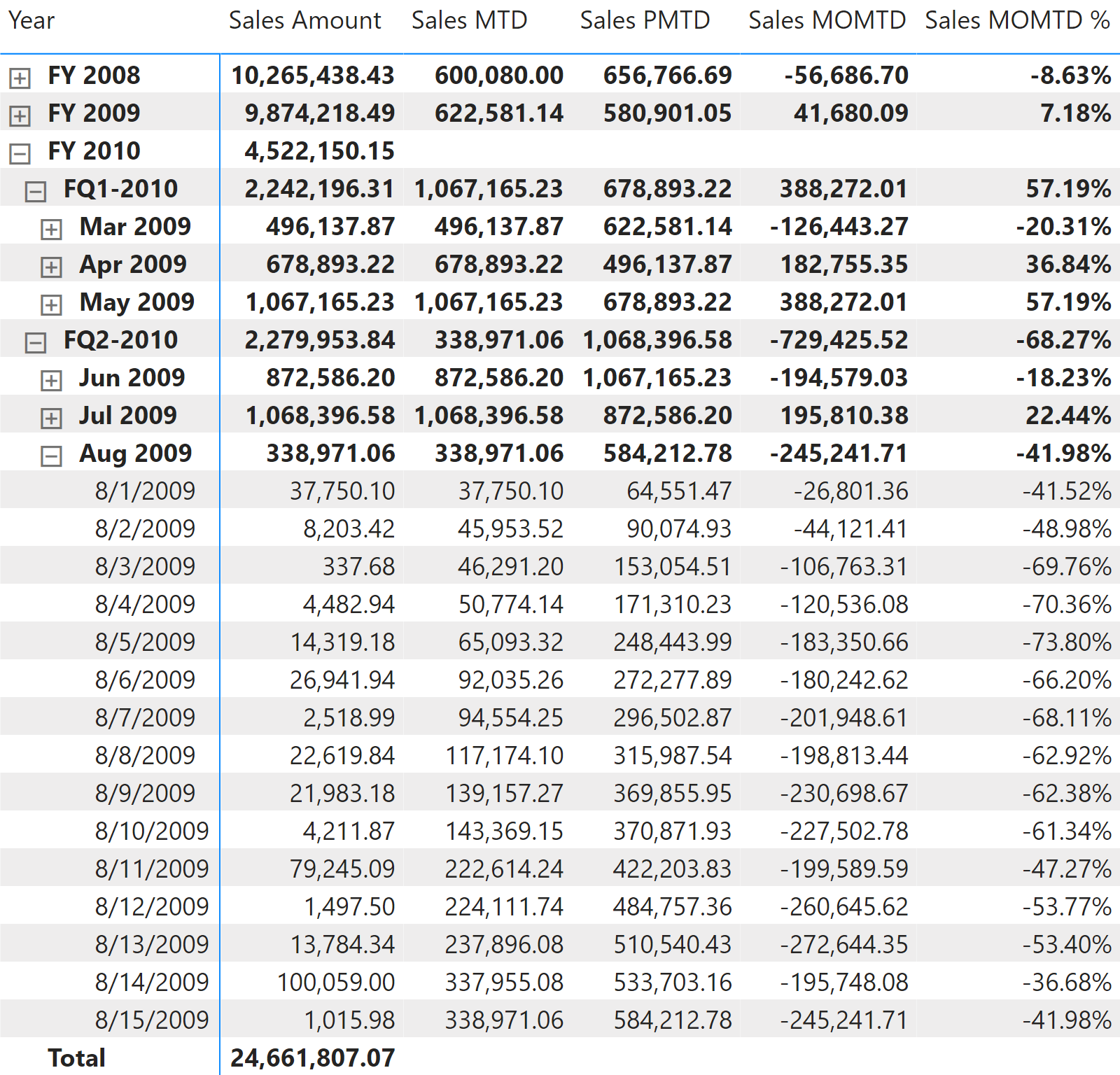
Month-over-month-to-date growth
Month-over-month-to-date growth compares a month-to-date at a specific date with the month-to-date at an equivalent date in the previous month. Figure 11 shows that Sales PMTD in August 2009 is only taking sales made up to July 15, 2009 into account, to get the corresponding portion of the previous month. For this reason Sales MTD of July 2009 is 1,068,396.58, whereas Sales PMTD for August 2009 is lower: 584,212.78.
Sales PMTD performs several steps, some of which are somewhat complex. The first two variables are quite easy: LastMonthSelected contains the last month visible in the filter context, while DaysOnLastMonth contains the number of days in LastMonthSelected.
It is important to note that if DaysOnLastMonth is equal to DaysLastMonthSelected, it means that the current filter context includes the end of a month; therefore the corresponding selection in the previous month must include the complete month. If DaysOnLastMonth is not equal to DaysLastMonthSelected, then the filter context is restricting the number of visible days. Consequently, we compute the last day of the month with data, and we restrict the result to only go up to the same day number in the previous month. This calculation takes place in LastDayOfMonthWithSales, which contains the last day of the month with sales data regardless of the filter-keep columns.
If the selection in the last month includes the whole month, then LastDayOfMonthWithSales contains the fixed value 31, which is a number greater than or equal to all the other days of a month. The LastDayOfMonthWithSales is then used to filter the days in the previous month, which is obtained by subtracting one to the value of LastMonthSelected:
Sales PMTD :=
IF (
    [ShowValueForDates],
    VAR LastMonthSelected =
        MAX ( 'Date'[Year Month Number] )
    VAR DaysOnLastMonth =
        CALCULATE (
            COUNTROWS ( 'Date' ),
            ALLEXCEPT ( 'Date', 'Date'[Working Day], 'Date'[Day of week] ),
            'Date'[Year Month Number] = LastMonthSelected
        )
    VAR DaysLastMonthSelected =
        CALCULATE (
            COUNTROWS ( 'Date' ),
            'Date'[DateWithSales] = TRUE,
            'Date'[Year Month Number] = LastMonthSelected
        )
    VAR LastDayOfMonthWithSales =
        MAX (
            -- End of month of any month
            31 * (DaysOnLastMonth = DaysLastMonthSelected),
            -- or last day selected with data
            CALCULATE (
                MAX ( 'Date'[Day of Month Number] ),
                REMOVEFILTERS (                -- Removes filters from all of the
                    'Date'[Working Day],       -- filter-keep columns
                    'Date'[Day of Week],       -- to get the last day with data
                    'Date'[Day of Week Number] -- selected in the report
                ),
                'Date'[Year Month Number] = LastMonthSelected,
                'Date'[DateWithSales] = TRUE
            )
        )
    VAR PreviousYearMonth =
        LastMonthSelected - 1
    VAR Result =
        CALCULATE (
            [Sales Amount],
            ALLEXCEPT ( 'Date', 'Date'[Working Day], 'Date'[Day of Week] ),
            'Date'[Year Month Number] = PreviousYearMonth,
            'Date'[Day of Month Number] <= LastDayOfMonthWithSales
        )
    RETURN
        Result
)
Sales MOMTD and Sales MOMTD % rely on the Sales PMTD measure to guarantee a fair comparison:
Sales MOMTD :=
VAR ValueCurrentPeriod = [Sales MTD]
VAR ValuePreviousPeriod = [Sales PMTD]
VAR Result =
    IF (
        NOT ISBLANK ( ValueCurrentPeriod )
            && NOT ISBLANK ( ValuePreviousPeriod ),
        ValueCurrentPeriod - ValuePreviousPeriod
    )
RETURN
    Result
Sales MOMTD % :=
DIVIDE (
    [Sales MOMTD],
    [Sales PMTD]
)
Comparing period-to-date with a previous full period
Comparing a to-date aggregation with the previous full time period is useful when you look at the previous period as a benchmark. Once the current year-to-date reaches 100% of the full previous year, this means you have reached the same performance as the previous full period, hopefully in fewer days.
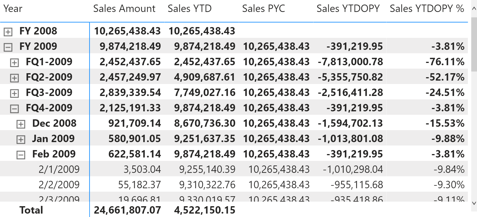
Year-to-date over the full previous year
The year-to-date over the full previous year compares the year-to-date against the entire previous year. Figure 12 shows that in January 2009 (which is close to the end of FY 2009) Sales YTD is 10% lower than Sales Amount for the entire fiscal year 2008. Sales YTDOPY % provides an immediate comparison of the year-to-date with the total of the previous year; it shows growth over the previous year when the percentage is positive, which never happens in this example.
The year-to-date-over-previous-year growth is computed by the Sales YTDOPY and Sales YTDOPY % measures; these rely on the Sales YTD measure to compute the year-to-date value, and on the Sales PYC measure to get the sales amount of the entire previous year:
Sales PYC :=
IF (
    [ShowValueForDates] && HASONEVALUE ( 'Date'[Fiscal Year Number] ),
    VAR PreviousFiscalYear = MAX ( 'Date'[Fiscal Year Number] ) - 1
    VAR Result =
        CALCULATE (
            [Sales Amount],
            ALLEXCEPT ( 'Date', 'Date'[Working Day], 'Date'[Day of Week] ),
            'Date'[Fiscal Year Number] = PreviousFiscalYear
        )
    RETURN
        Result
)
Sales YTDOPY :=
VAR ValueCurrentPeriod = [Sales YTD]
VAR ValuePreviousPeriod = [Sales PYC]
VAR Result =
    IF (
        NOT ISBLANK ( ValueCurrentPeriod )
            && NOT ISBLANK ( ValuePreviousPeriod ),
        ValueCurrentPeriod - ValuePreviousPeriod
    )
RETURN
    Result
Sales YTDOPY % :=
DIVIDE (
    [Sales YTDOPY],
    [Sales PYC]
)
Quarter-to-date over the full previous quarter
The quarter-to-date over the full previous quarter compares the quarter-to-date against the entire previous quarter. Figure 13 shows that Sales QTD surpassed the total Sales Amount for FQ1-2008 only in August 2008. Sales QTDOPQ % provides an immediate comparison of the quarter-to-date with the total of the previous quarter; it shows growth over the previous quarter when the percentage is positive.
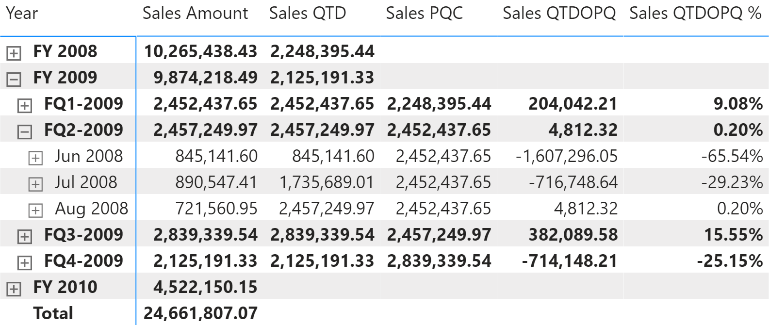
The quarter-to-date-over-previous-quarter growth is computed with the Sales QTDOPQ and Sales QTDOPQ % measures; these rely on the Sales QTD measure to compute the quarter-to-date value and on the Sales PQC measure to get the sales amount of the entire previous quarter:
Sales PQC :=
IF (
    [ShowValueForDates] && HASONEVALUE ( 'Date'[Fiscal Year Quarter Number] ),
    VAR PreviousFiscalYearQuarter = MAX ( 'Date'[Fiscal Year Quarter Number] ) - 1
    VAR Result =
        CALCULATE (
            [Sales Amount],
            ALLEXCEPT ( 'Date', 'Date'[Working Day], 'Date'[Day of Week] ),
            'Date'[Fiscal Year Quarter Number] = PreviousFiscalYearQuarter
        )
    RETURN
        Result
)
Sales QTDOPQ :=
VAR ValueCurrentPeriod = [Sales QTD]
VAR ValuePreviousPeriod = [Sales PQC]
VAR Result =
    IF (
        NOT ISBLANK ( ValueCurrentPeriod )
            && NOT ISBLANK ( ValuePreviousPeriod ),
        ValueCurrentPeriod - ValuePreviousPeriod
    )
RETURN
    Result
Sales QTDOPQ % :=
DIVIDE (
    [Sales QTDOPQ],
    [Sales PQC]
)
Month-to-date over the full previous month
The month-to-date over the full previous month compares the month-to-date against the entire previous month. Figure 14 shows that Sales MTD during April 2008 surpasses the total Sales Amount for March 2008. Sales MTDOPM % provides an immediate comparison of the month-to-date with the total of the previous month; it shows growth over the previous month when the percentage is positive as is the case starting April 19, 2008.
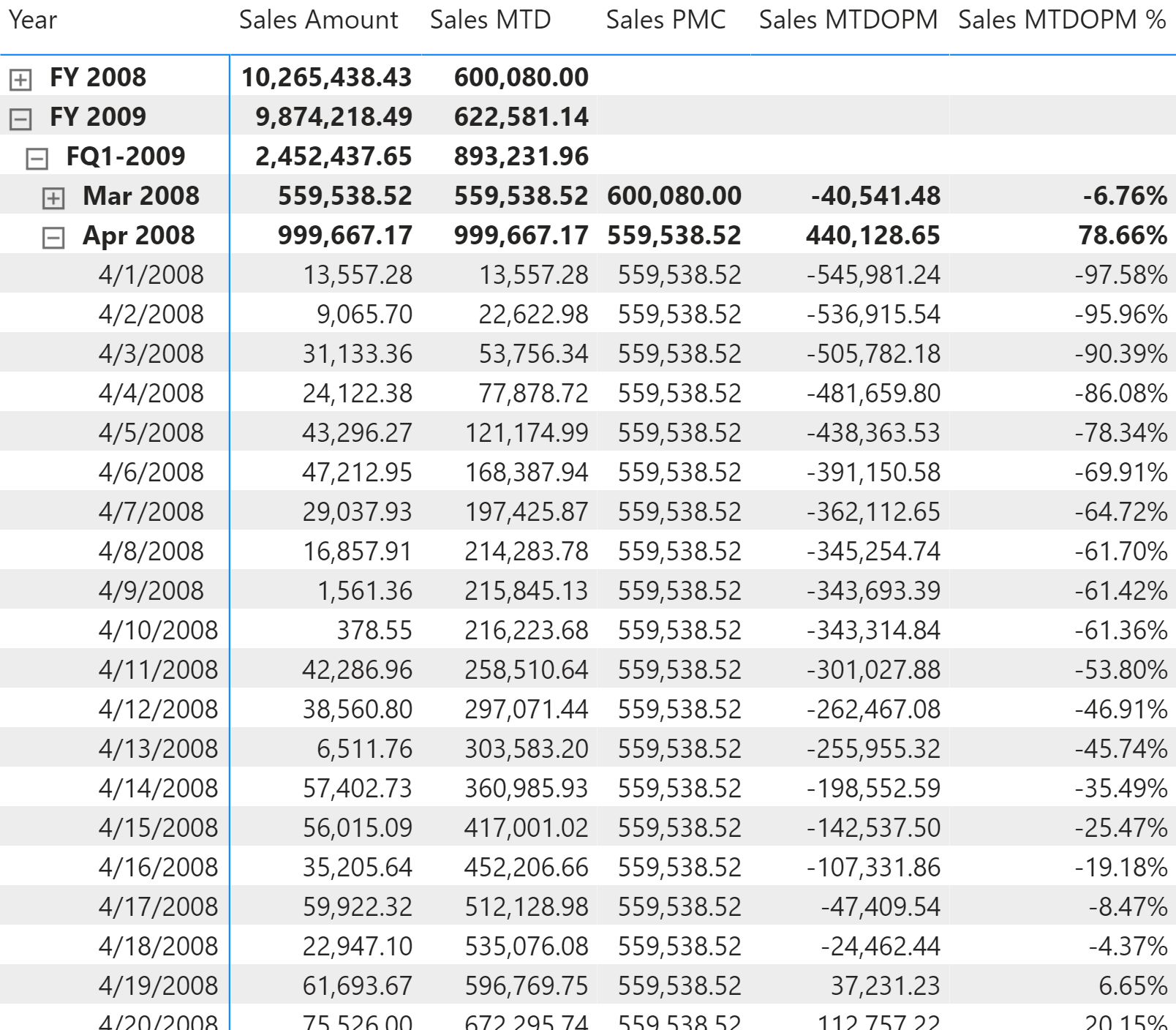
The month-to-date-over-previous-month growth is computed with the Sales MTDOPM % and Sales MTDOPM measures; these rely on the Sales MTD measure to compute the month-to-date value and on the Sales PMC measure to get the sales amount of the entire previous month:
Sales PMC :=
IF (
    [ShowValueForDates] && HASONEVALUE ( 'Date'[Year Month Number] ),
    VAR PreviousFiscalYearMonth = MAX ( 'Date'[Year Month Number] ) - 1
    VAR Result =
        CALCULATE (
            [Sales Amount],
            ALLEXCEPT ( 'Date', 'Date'[Working Day], 'Date'[Day of Week] ),
            'Date'[Year Month Number] = PreviousFiscalYearMonth
        )
    RETURN
        Result
)
Sales MTDOPM :=
VAR ValueCurrentPeriod = [Sales MTD]
VAR ValuePreviousPeriod = [Sales PMC]
VAR Result =
    IF (
        NOT ISBLANK ( ValueCurrentPeriod )
            && NOT ISBLANK ( ValuePreviousPeriod ),
        ValueCurrentPeriod - ValuePreviousPeriod
    )
RETURN
    Result
Sales MTDOPM % :=
DIVIDE (
    [Sales MTDOPM],
    [Sales PMC]
)
Using moving annual total calculations
A common way of aggregating data over several months is by using the moving annual total instead of the year-to-date. The moving annual total includes the last 12 months of data. For example, the moving annual total for March 2008 includes data from April 2007 to March 2008.
Moving annual total
Sales MAT computes the moving annual total, as shown in Figure 15. The same report also shows Sales MAT (364): it is a similar measure with the difference that it uses the last 364 days (corresponding to the last 52 weeks), instead of a full year.
The Sales MAT measure defines a range over the Date[Date] column that includes the days of one complete year starting from the last day in the filter context:
Sales MAT :=
IF (
    [ShowValueForDates],
    VAR LastDayMAT =  MAX ( 'Date'[Sequential Day Number] )
    VAR FirstDayMAT = INT ( EDATE ( LastDayMAT + 1, -12 ) )
    VAR Result =
        CALCULATE (
            [Sales Amount],
            ALLEXCEPT ( 'Date', 'Date'[Working Day], 'Date'[Day of Week] ),
            'Date'[Sequential Day Number] >= FirstDayMAT
                && 'Date'[Sequential Day Number] <= LastDayMAT
        )
    RETURN
        Result
)
Sales MAT (364) does not correspond to a total over the year. Yet, it is a good measure to evaluate trends over time or in a chart because it always includes the same number of days and an integer number of weeks. Consequently, the days of the week are evenly represented in the result. The measure defines a range over the Date[Date] column that includes the last 364 days from the last day in the filter context:
Sales MAT (364) :=
IF (
    [ShowValueForDates],
    VAR LastDayMAT =  MAX ( 'Date'[Sequential Day Number] )
    VAR FirstDayMAT = LastDayMAT - 363
    VAR Result =
        CALCULATE (
            [Sales Amount],
            ALLEXCEPT ( 'Date', 'Date'[Working Day], 'Date'[Day of Week] ),
            'Date'[Sequential Day Number] >= FirstDayMAT
                && 'Date'[Sequential Day Number] <= LastDayMAT
        )
    RETURN
        Result
)
Moving annual total growth
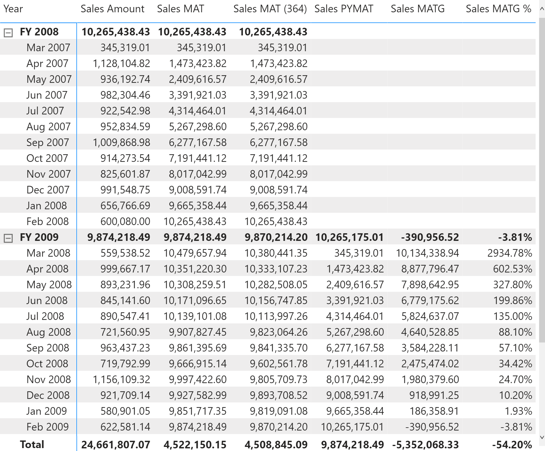
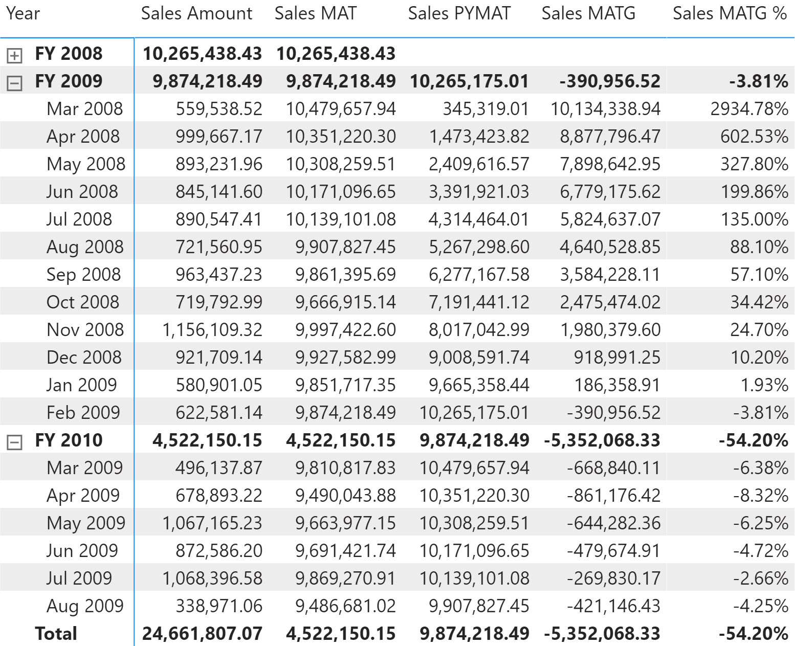
The moving annual total growth is computed with the Sales PYMAT, Sales MATG, and Sales MATG % measures, which rely on the Sales MAT measure. The Sales MAT measure provides a correct value one year after the first sale ever (when it collects one full year of data), and it is not protected in case the current time period is shorter than a full year. For example, the amount for the fiscal year 2010 of Sales PYMAT is 9,874,218.49, which corresponds to the Sales Amount of FY 2009 as shown in Figure 16. When compared with sales in FY 2010, this produces a comparison of less than 6 months – data being only available until August 15, 2009 – with the full fiscal year 2009. Similarly, you can see that Sales MATG % starts in FY 2009 with very high values and stabilizes after a year. This behavior is by design: the moving annual total is usually computed at the month or day granularity to show trends in a chart.
The measures are defined as follows:
Sales PYMAT :=
IF (
    [ShowValueForDates],
    VAR LastDayAvailable = MAX ( 'Date'[Sequential Day Number] )
    VAR LastDayMAT =  INT ( EDATE ( LastDayAvailable, -12 ) )
    VAR FirstDayMAT = INT ( EDATE ( LastDayAvailable + 1, -24 ) )
    VAR Result =
        CALCULATE (
            [Sales Amount],
            ALLEXCEPT ( 'Date', 'Date'[Working Day], 'Date'[Day of Week] ),
            'Date'[Sequential Day Number] >= FirstDayMAT
                && 'Date'[Sequential Day Number] <= LastDayMAT
        )
    RETURN
        Result
)
Sales MATG :=
VAR ValueCurrentPeriod = [Sales MAT]
VAR ValuePreviousPeriod = [Sales PYMAT]
VAR Result =
    IF (
        NOT ISBLANK ( ValueCurrentPeriod )
            && NOT ISBLANK ( ValuePreviousPeriod ),
        ValueCurrentPeriod - ValuePreviousPeriod
    )
RETURN
    Result
Sales MATG % :=
DIVIDE (
    [Sales MATG],
    [Sales PYMAT]
)
The Sales PYMAT measure can also be written using the last 364 days, similar to Sales MAT (364) – the difference between Sales PYMAT and Sales PYMAT (364) is the evaluation of the FirstDayMAT and the LastDayMAT variables:
Sales PYMAT (364) :=
IF (
    [ShowValueForDates],
    VAR LastDayAvailable = MAX ( 'Date'[Sequential Day Number] )
    VAR LastDayMAT = LastDayAvailable - 364
    VAR FirstDayMAT = LastDayMAT - 363
    VAR Result =
        CALCULATE (
            [Sales Amount],
            ALLEXCEPT ( 'Date', 'Date'[Working Day], 'Date'[Day of Week] ),
            'Date'[Sequential Day Number] >= FirstDayMAT
                && 'Date'[Sequential Day Number] <= LastDayMAT
        )
    RETURN
        Result
)
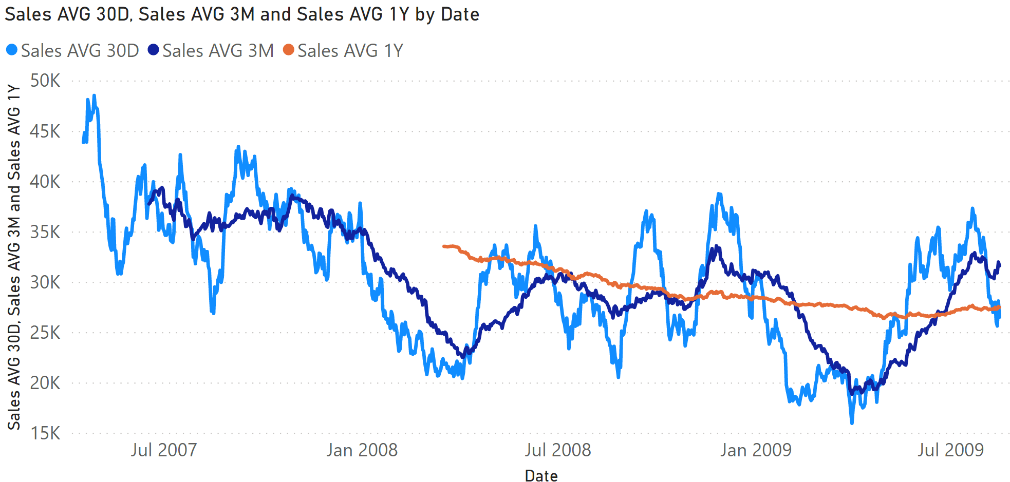
Moving averages
The moving average is typically used to display trends in line charts. Figure 17 includes the moving average of Sales Amount over 30 days (Sales AVG 30D), three months (Sales AVG 3M), and a year (Sales AVG 1Y).
Moving average 30 days
The Sales AVG 30D measure computes the moving average over 30 days by iterating a list of the last 30 dates obtained in the Period30D variable. It does so by fetching the dates visible included in the last 30 days, while ignoring dates without sales and taking into account filters applied by filter-keep columns in the Date table:
Sales AVG 30D :=
IF (
    [ShowValueForDates],
    VAR LastDayMAT =
        MAX ( 'Date'[Sequential Day Number] )
    VAR FirstDayMAT = LastDayMAT - 29
    VAR Period30D =
        CALCULATETABLE (
            VALUES ( 'Date'[Sequential Day Number] ),
            ALLEXCEPT (
                'Date',
                'Date'[Working Day],
                'Date'[Day of Week]
            ),
            'Date'[Sequential Day Number] >= FirstDayMAT
                && 'Date'[Sequential Day Number] <= LastDayMAT,
            'Date'[DateWithSales] = TRUE
        )
    VAR FirstDayWithData =
        CALCULATE (
            INT ( MIN ( Sales[Order Date] ) ),
            REMOVEFILTERS ()
        )
    VAR FirstDayInPeriod =
        MINX (
            Period30D,
            'Date'[Sequential Day Number]
        )
    VAR Result =
        IF (
            FirstDayWithData <= FirstDayInPeriod,
            CALCULATE (
                AVERAGEX ( Period30D, [Sales Amount] ),
                REMOVEFILTERS ( 'Date' )
            )
        )
    RETURN
        Result
)
This pattern is very flexible because it also works for non-additive measures. With that said, for a regular additive calculation Result can be implemented using a different and faster formula:
VAR Result =
    IF (
        FirstDayWithData <= FirstDayInPeriod,
        CALCULATE (
            DIVIDE (
                [Sales Amount],
                DISTINCTCOUNT ( Sales[Order Date] )
            ),
            Period30D,
            REMOVEFILTERS ( 'Date' )
        )
    )
Moving average 3 months
The Sales AVG 3M measure computes the moving average over three months. It iterates a list of the dates in the last three months obtained in the Period3M variable by getting the dates visible included in the last 3 months, by ignoring dates without sales and by taking into account the filters applied by filter-keep columns in the Date table:
Sales AVG 3M :=
IF (
    [ShowValueForDates],
    VAR LastDayMAT =
        MAX ( 'Date'[Sequential Day Number] )
    VAR FirstDayMAT =
        INT ( EDATE ( LastDayMAT + 1, -3 ) )
    VAR Period3M =
       CALCULATETABLE (
            VALUES ( 'Date'[Sequential Day Number] ),
            ALLEXCEPT (
                'Date',
                'Date'[Working Day],
                'Date'[Day of Week]
            ),
            'Date'[Sequential Day Number] >= FirstDayMAT
                && 'Date'[Sequential Day Number] <= LastDayMAT,
            'Date'[DateWithSales] = TRUE
        )
    VAR FirstDayWithData =
        CALCULATE (
            INT ( MIN ( Sales[Order Date] ) ),
            REMOVEFILTERS ()
        )
    VAR FirstDayInPeriod =
        MINX (
            Period3M,
            'Date'[Sequential Day Number]
        )
    VAR Result =
        IF (
            FirstDayWithData <= FirstDayInPeriod,
            CALCULATE (
                AVERAGEX ( Period3M, [Sales Amount] ),
                REMOVEFILTERS ( 'Date' )
            )
        )
    RETURN
        Result
)
For simple additive measures, the pattern based on DIVIDE which is shown for the moving average over 30 days can also be used for the average over three months.
Moving average 1 year
The Sales AVG 1Y measure computes the moving average over one year by iterating a list of the dates in the last year in the Period1Y variable. It does so by getting the dates visible included in the last year, by ignoring dates without sales and by taking into account filters applied by filter-keep columns in the Date table:
Sales AVG 1Y :=
IF (
    [ShowValueForDates],
    VAR LastDayMAT =
        MAX ( 'Date'[Sequential Day Number] )
    VAR FirstDayMAT =
        INT ( EDATE ( LastDayMAT + 1, -12 ) )
    VAR Period1Y =
        CALCULATETABLE (
            VALUES ( 'Date'[Sequential Day Number] ),
            ALLEXCEPT (
                'Date',
                'Date'[Working Day],
                'Date'[Day of Week]
            ),
            'Date'[Sequential Day Number] >= FirstDayMAT
                && 'Date'[Sequential Day Number] <= LastDayMAT,
            'Date'[DateWithSales] = TRUE
        )
    VAR FirstDayWithData =
        CALCULATE (
            INT ( MIN ( Sales[Order Date] ) ),
            REMOVEFILTERS ()
        )
    VAR FirstDayInPeriod =
        MINX (
            Period1Y,
            'Date'[Sequential Day Number]
        )
    VAR Result =
        IF (
            FirstDayWithData <= FirstDayInPeriod,
            CALCULATE (
                AVERAGEX ( Period1Y, [Sales Amount] ),
                REMOVEFILTERS ( 'Date' )
            )
        )
    RETURN
        Result
)
For simple additive measures, the pattern based on DIVIDE shown for the moving average over 30 days can also be used for the average over one year.
Returns a table that has been filtered.
FILTER ( <Table>, <FilterExpression> )
Evaluates an expression in a context modified by filters.
CALCULATE ( <Expression> [, <Filter> [, <Filter> [, … ] ] ] )
Clear filters from the specified tables or columns.
REMOVEFILTERS ( [<TableNameOrColumnName>] [, <ColumnName> [, <ColumnName> [, … ] ] ] )
Returns all the rows in a table except for those rows that are affected by the specified column filters.
ALLEXCEPT ( <TableName>, <ColumnName> [, <ColumnName> [, … ] ] )
Returns true when the specified column is the level in a hierarchy of levels.
ISINSCOPE ( <ColumnName> )
The IsOnOrAfter function is a boolean function that emulates the behavior of Start At clause and returns true for a row that meets all the conditions mentioned as parameters in this function.
ISONORAFTER ( <Value1>, <Value2> [, [<Order>] [, <Value1>, <Value2> [, [<Order>] [, … ] ] ] ] )
Safe Divide function with ability to handle divide by zero case.
DIVIDE ( <Numerator>, <Denominator> [, <AlternateResult>] )
This pattern is included in the book DAX Patterns, Second Edition.


Video

Do you prefer a video?
This pattern is also available in video format. Take a peek at the preview, then unlock access to the full-length video on SQLBI.com.Watch the full video — 100 min.
Downloads
Download the sample files for Power BI / Excel 2016-2019: